Modified from a Jeffrey Beall photo, via Flickr (CC-BY)
LEARNING OBJECTIVES
After reading this chapter, students should be able to:
- Identify the causal mechanisms and ecological ramifications of each of the Big Five mass extinctions that have occurred in geologic time
- Describe several smaller biotic transitions that have significantly impacted the diversity of life on Earth through geologic time
Adaptation’s dark twin
Natural selection and related processes control the evolution of organic life. Elsewhere in this text, we have explored how random mutations in the genetic material inside organisms’ cells produces variations in their size, shape, and abilities, some of which will provide a selective advantage over other individuals. In those circumstances, the mutated individual is likely to enjoy enhanced survival, and thus enhanced reproduction, which passes the gene for the new trait on to the next generation. The new trait is an adaptation. Through repeated cycles of copying and culling, the adaptive gene spreads through the population and comes to dominate. If the changes are sufficiently pronounced, we call the organism by a different name; we infer that speciation (or “origination”) has occurred.
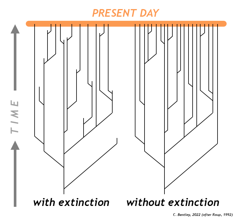
Callan Bentley redrawing of an original diagram by David Raup.
However, this narrative emphasizes the spread of a new trait (and the gene that codes for it). Equally critical in the history of life is the cancellation of some old traits (and the genes that code for them). Without extinction, there would likely be insufficient ecological “space” available for new species. The pattern we see in the fossil record is not one of continuous diversification with new species being added, but none ever removed. Instead, the average species lasts a few million years, and then vanishes forever from the face of the planet. It goes extinct. A handful of species have persisted with relatively minimal change (sometimes we call them “living fossils”), but most lineages show changes through time, gaining some species but losing others. As you look around the world today and (rightly) marvel at the diversity of organisms who share your planet with you, it is sobering to realize that Earth’s deep time hosted many, many more — species that got snuffed out somewhere along the way. Estimates are that 99.9% of all species that ever existed on Earth no longer exist — the vast majority have gone extinct. Most of these occur as part of the normal “background extinction” rate, a regular coming-and-going of species due to habitat loss, changing physical environments, and biologic pressures over time.
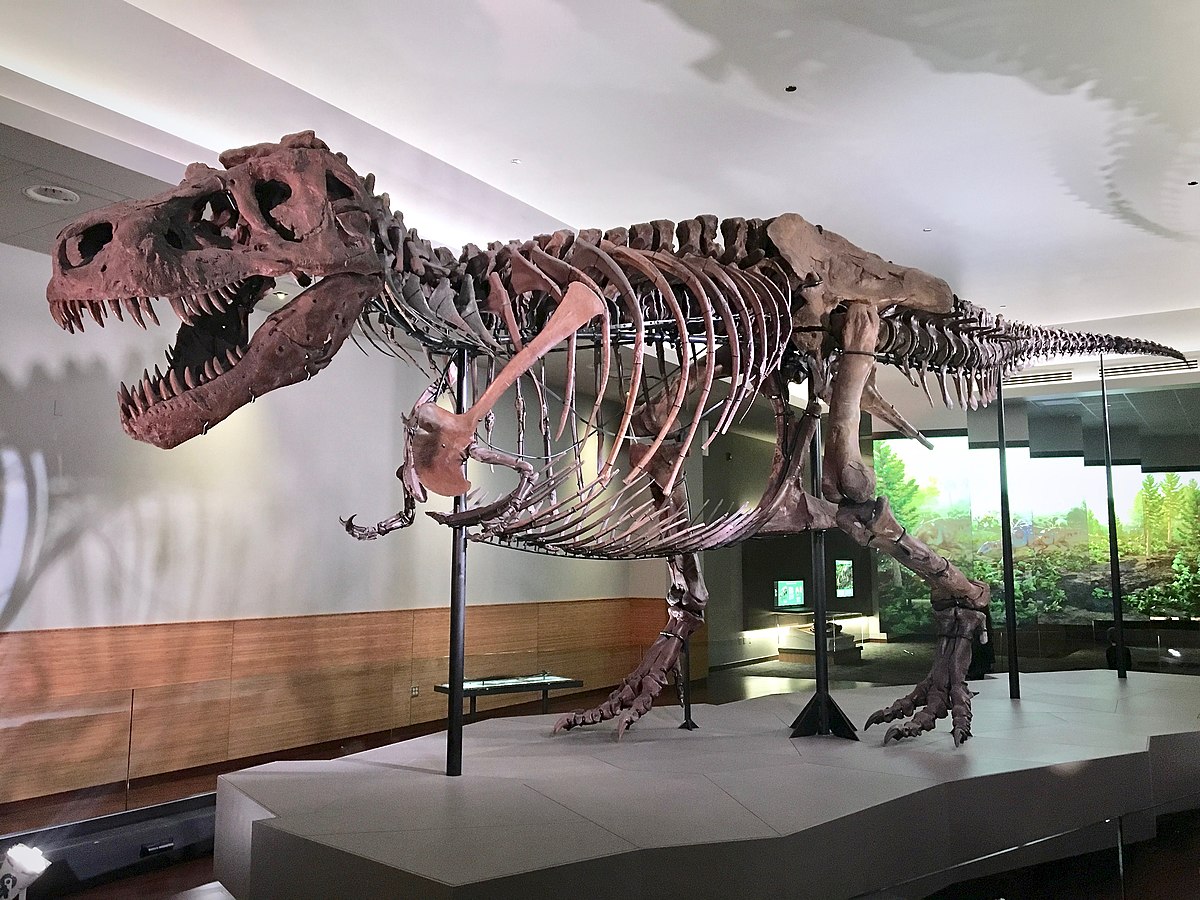
Periodically, entire lineages will go extinct. The trilobites, for instance, were exceptionally diverse and widespread, but they never made it out of Paleozoic Era. Similarly, sauropod dinosaurs are a Mesozoic-only group. When multiple lines of descent all terminate at the same moment in geologic time, we call it a mass extinction. Mass extinctions potentially imply a common cause for the synchronous extinctions of many unrelated groups. We study mass extinctions because they are fascinating and dramatic, but also because we worry about our own future. The study of mass extinctions demonstrate that Earth’s biosphere can periodically be wrecked, and then healed, but healed with a new suite of organisms. Put another way, every time there is a mass extinction episode, it is followed by a time when the survivors diversify and adapt, taking advantage of the lack of competition. This is an adaptive radiation. For instance, after the reptilian dinosaurs, mosasaurs, and pterosaurs went extinct at the end of the Cretaceous, mammals underwent an adaptive radiation, diversifying to fill all sorts of ecological niches on land, sea, and even in the air.
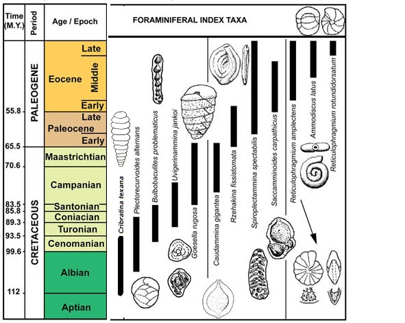
For educational purposes from the Geologic Timescale Foundation. Modified by Shelley Jaye.
We know about mass extinctions because of careful study of the appearance of fossil forms in the stratigraphic record. Each species has a geologic range defined by its first appearance (oldest stratum in which it is known) and its last appearance (youngest stratum in which it is known). Like any scientific conclusion, these ranges are always subject to change with new data (such as in the famous case of the coelacanth), but for the most part the ranges are well established, having stood repeated testing over the past two centuries of paleontological documentation.
Mass extinctions lead to declines in both diversity and abundance of organisms, are typically global scale events, and cut across taxonomic groups affecting organisms in a wide array of environmental habitats.
“The Big Five”
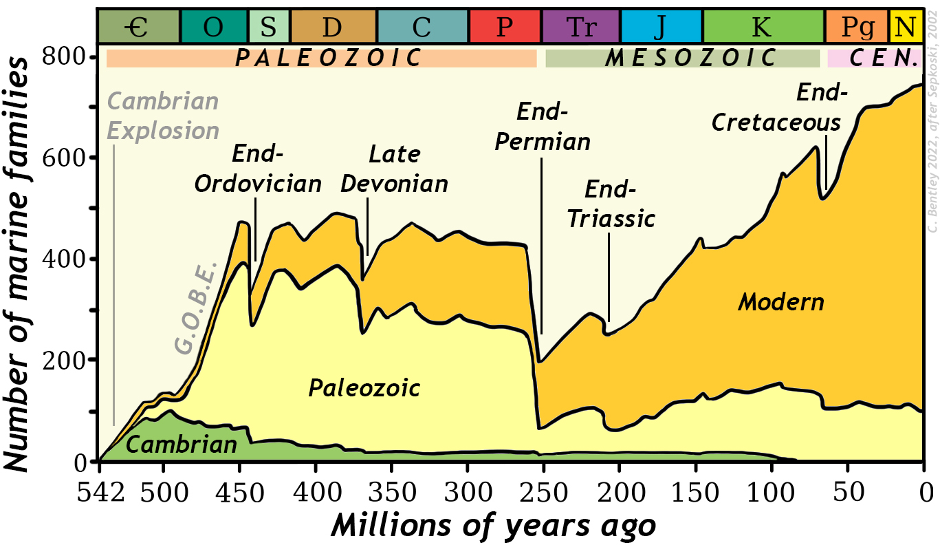
Graph by Callan Bentley (2022), after Sepkoski (1984, 2002).
Traditionally, historical geologists have recognized five major episodes of mass extinction from the fossil record. They show as big spikes on the graph above. Plotted a different way, they show as sharp declines on the diversity through time graph. Chronologically, they are the end-Ordovician extinction, the late Devonian, the end-Permian (which closes the Paleozoic Era), the end-Triassic, and the end-Cretaceous (which closes the Mesozoic Era). Each has its own idiosyncratic circumstances, cast of characters, and potentially unique causes for so much dying. Let us now recap each of them.
Extinction is going on all the time. In a way, it’s arbitrary to select a handful for consideration, both because of the incomplete nature of the fossil record (such as microbial turnover during the Great Oxygenation Event) and background extinctions (such as the spikes you see in the Cambrian above, which seem big because the total known number of fossil organisms was itself low).
End-Ordovician extinction
At the end of the Ordovician period, the only animals on Earth were invertebrates living in the ocean. Certain varieties of mollusks, trilobites, graptolites, eurypterids, brachiopods, conodonts, corals, echinoderms, and other groups all went extinct about 443 Ma. These were all key members of the Paleozoic Fauna. Of the species paleontologists have documented, about 52% of them disappeared at the Ordovician/Silurian boundary, never to return. It is worth emphasizing that — uniquely among the Big Five — the end-Ordovician extinction was entirely limited to marine organisms, since land had yet to be colonized at that time.
The Ordovician/Silurian boundary was defined by Charles Lapworth with the stratotype at Dob’s Linn, Scotland, which is still used as a GSSP today. Below are some of the graptolites Lapworth used as index fossils to distinguish between the two periods in the black shale there:
Callan Bentley GIGAmacro
After the mass extinction was over, it took 50 million years for Earth’s oceans to recover their former levels of diversity.
Modified from Figure 3 of Masri (2017).
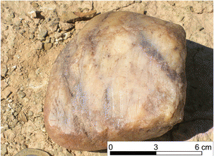
The cause of the late Ordovician extinction is inferred to likely be global cooling. There is evidence of glaciation during the late Ordovician in the southern supercontinent Gondwana: this is known from sedimentological documentation of tillites bearing faceted, striated clasts, and dropstones in what is today South America, Arabia and Africa). There are also vast areas where the glaciers appear to have bulldozed pre-existing unlithified sediments, deforming them as the ice flowed along. Using isotopic evidence, Finnegan et al. (2011) have estimated that global seawater temperatures dropped 5°C during the latest Ordovician. Five degrees may not sound like much, but because of water’s exceptional heat capacity and the huge volume of Earth’s seawater, it represents a truly enormous amount of heat energy lost from the world ocean. Glass sponges, a deep-water siliceous sponge-like animal, are well-adapted to cold conditions, and they do well in the aftermath of the end-Ordovician extinction.
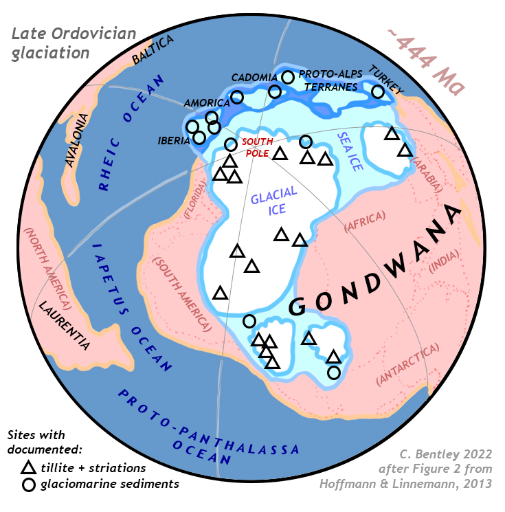
Map by Callan Bentley, redrawn after an original by Hoffmann and Linnemann, 2013.
How could a cooling climate trigger a mass extinction? One key variable is a change in the ocean temperature, with negative impacts for those organisms who are specialized for warmer waters. This is particularly acute in the tropical/equatorial regions of the planet’s ocean. But another key impact is in the change in sea level that accompanies the build up of glacial ice mass. Glaciers are made of water, and that water has to come from somewhere. As we are currently seeing in modern times, melting glaciers add water to the ocean, which raises sea level. The reverse is also true: at the height of the most recent ice age [LINK HERE TO PLEISTOCENE CASE STUDY], sea level was ~120 meters lower, and the shoreline was at the edge of the continental shelf. This is bad news for marine invertebrates, most of which live in the shallow marine realm. Dropping sea level by more than 330 feet reduces the amount of habitat they have in which to dwell, and increases competition between individuals.
What caused the cooling climate? It appears to be a coincidence of several events: (1) the position of Gondwana over the south polar region, drifting there due to plate tectonics, and (2) a lowering of greenhouse gas levels through some perturbation to the climate. We can break condition “2” down further into a couple of hypotheses: (2a) enhanced silicate weathering by rainwater carbonic acid due to an episode of mountain-building in ancestral North America, the Taconian Orogeny, and (2b) reduced sunlight influx due to stratospheric dust kicked up by a series of meteorite impacts. These aren’t necessarily mutually exclusive, of course. Let’s briefly examine each.
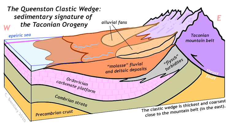
Callan Bentley cartoon.
The Taconian Orogeny, first phase of the three-part suite of Appalachian Orogenies, was caused by the collision of a volcanic island arc in the Iapetus Ocean with the Iapetan margin of ancestral North America. This raised a big chain of mountains that stretched from Maine to Georgia, and shed a tremendous quantity of clastic sediment, including a lot of mud. Mud is made mainly of clay minerals, which are produced through the hydrolysis of feldspars. Mountain belts put a lot of feldspar into the path of chemical weathering, which gobbles up CO2 from the atmosphere.
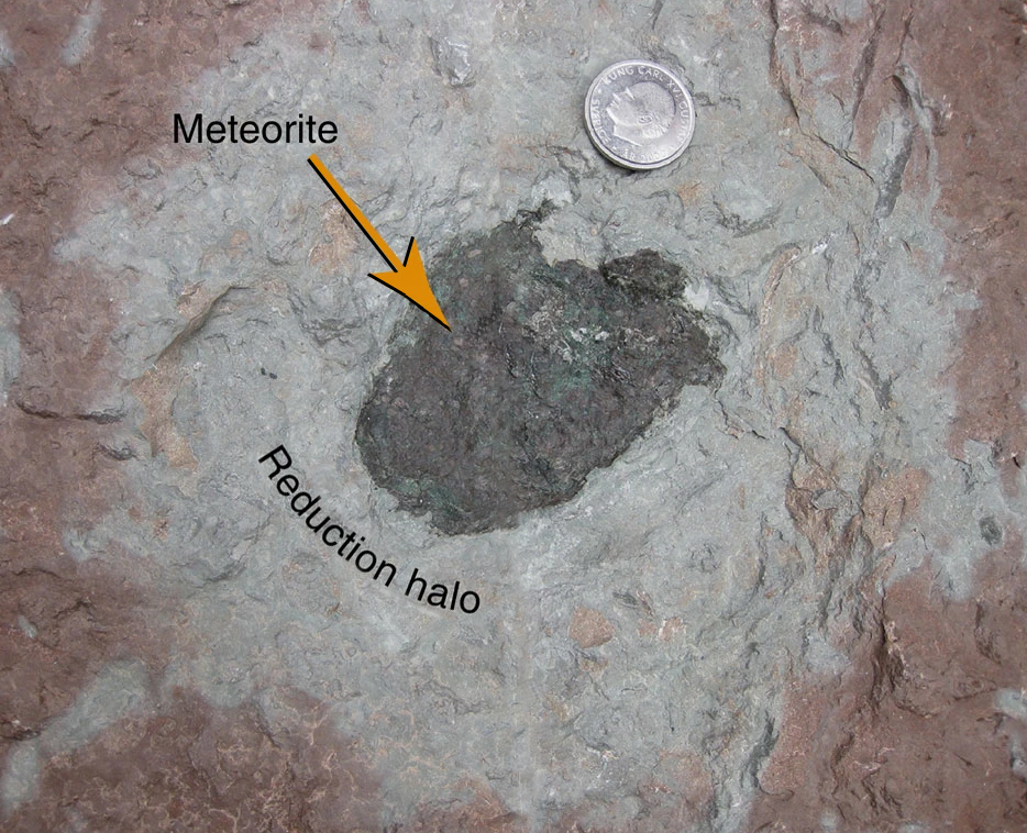
Modified (enhanced!) by CB from an original by Shmitz, et al. 2016.
Another possibility has an extraterrestrial component. For a long time, it was observed in limestone quarries in Sweden that there were a lot of meteorites included in those carbonate strata. More widely and generally, sedimentary rocks of that time contained a lot of chromite grains that were attributed to meteors. These meteorites generally share a common composition; they are classified as “L-chondrites,” and are all inferred to come from the breakup of a single chondritic parent body, floating somewhere out in space, at about 468 Ma. There are a lot of them; the profusion of meteorites and chromite grains has been dubbed the Ordovician Meteor Event. The idea is that these meteorites would have kicked up a lot of dust. If that dust reached the stratosphere, where there is no rain or weather, then it could have blocked incoming sunlight. A reduction in the flux of sunlight would have acted to cool the climate, regardless of what greenhouse gases were doing at the time of impact.
So, to summarize: it looks like the first of the Big Five mass extinctions was driven by global cooling.
Late Devonian extinction

Public domain.
After the relatively brief Silurian period (total duration only 20 million years), the planet entered the Devonian period, sometimes dubbed “the age of fishes.” This was a time of great radiation among the fishes, producing the first jawless fishes, sharks, placoderms, the first ray-finned fish, and the lobe-finned fishes, some of whom were almost certainly the ancestors of the humans reading this case study.
Drawing by Phillipe Janvier (1997), CC-BY.
Toward the end of the Devonian, things started getting rough for organisms on Earth, but unlike the end-Ordovician, end-Permian, end-Triassic, and end-Cretaceous extinctions, this one took a while. It was spread out over more than 20 million years, maybe as many as 25 million. It’s not the called the “end”-Devonian, for that reason. It took a while. It got worse, and then a little better, and then worse again. The two biggest die-offs occurred at 374 Ma and 359 Ma.
Dwergenpaartje photo, CC-BY, via Wikimedia.
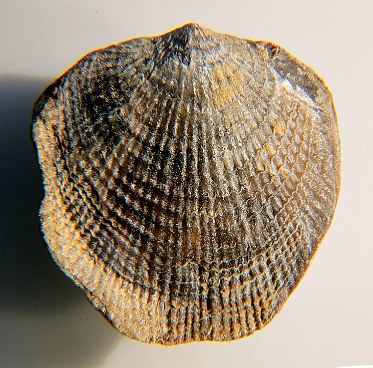
By the end of it, though, 99% of reefs had been destroyed, the diverse fish world had been severely cut back, and many marine groups had been severely pruned back or eliminated altogether. Among reef-builders, the tabulate and rugose corals got slammed. Conservative estimates put the carnage at a 40% loss of taxa. The atrypid brachiopods, for instance, were a diverse tropical group of articulate brachiopods that were extinguished. Moving into their shallow-sea habitat after the extinction were silica-skeleton sponges, which otherwise prefer cooler, deeper water.
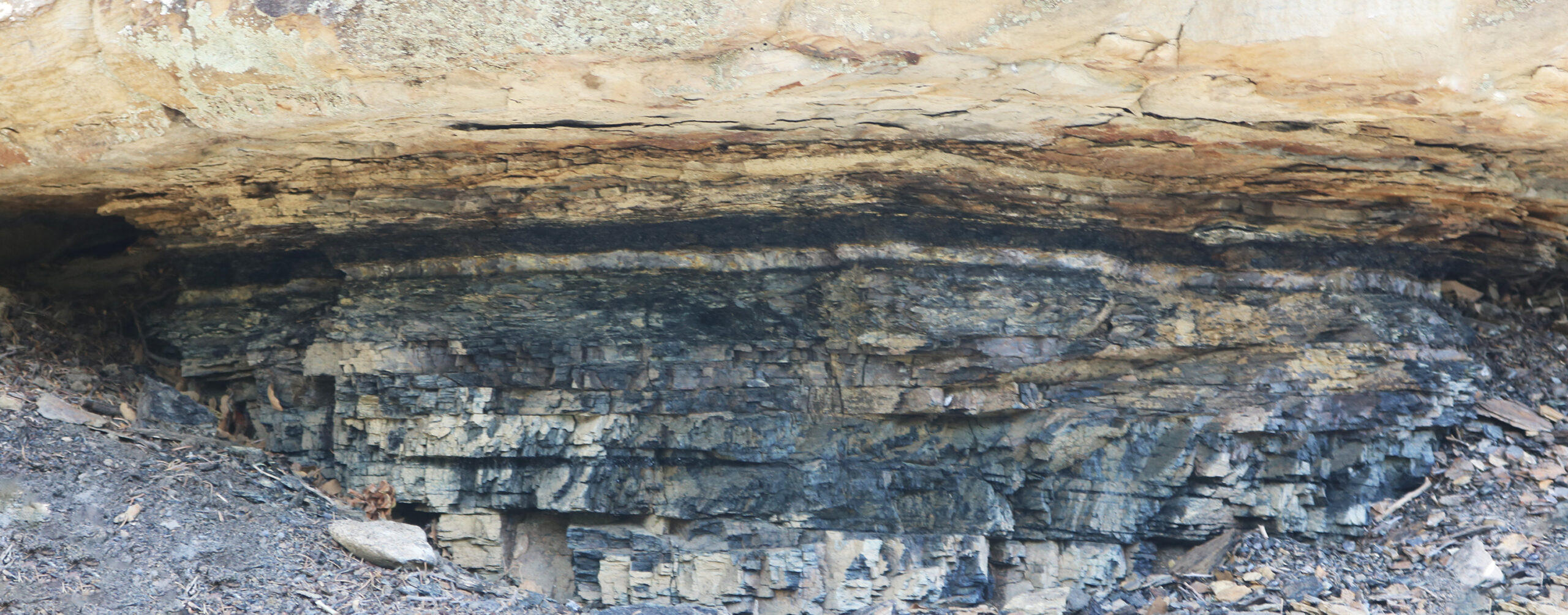
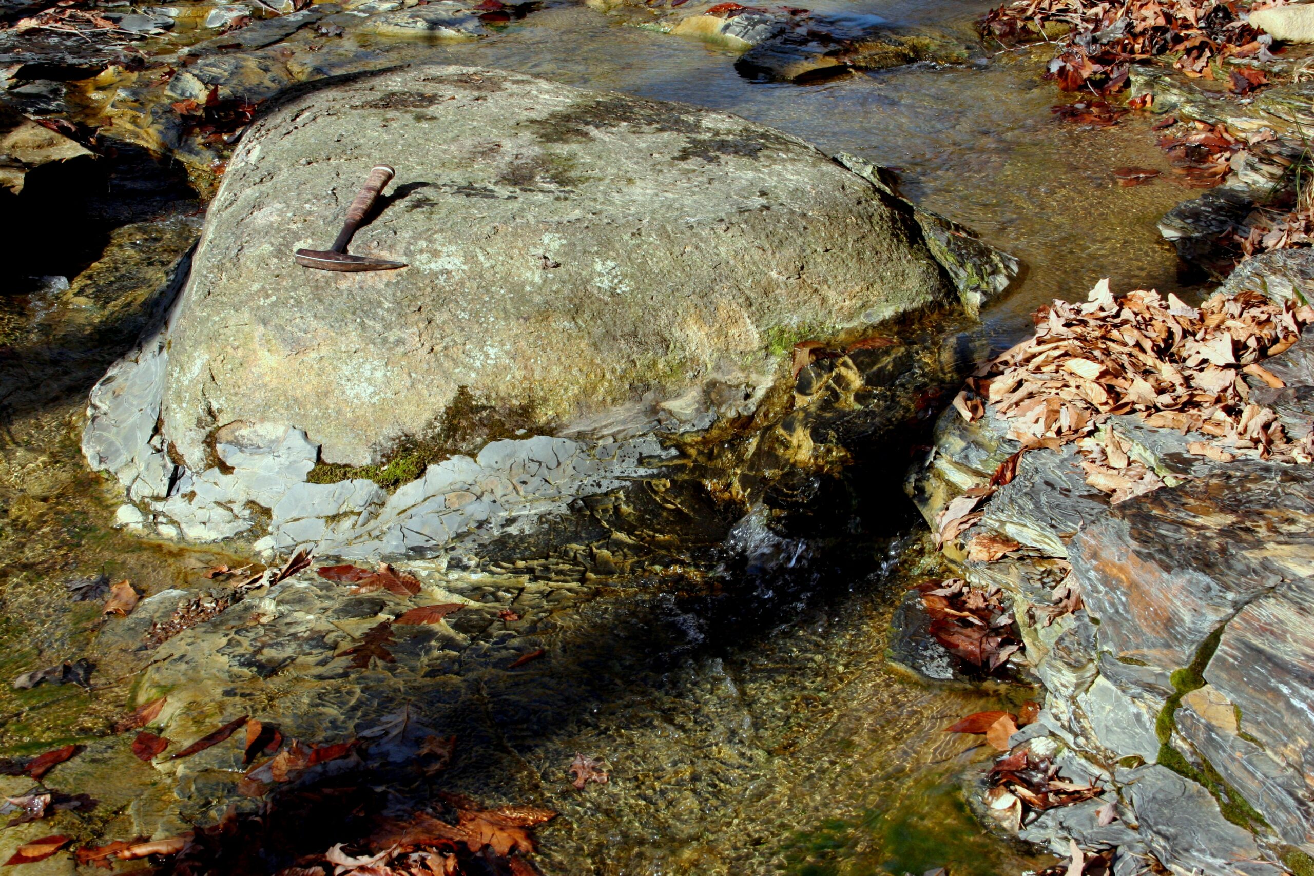
One of the first clues that things were going awry in the late Devonian is a profusion of black shales. Black shale is rich in organic carbon.

Photograph by Barbara Friedman, CC-BY, via Flickr.
Carbon loves to react with oxygen, if there’s any oxygen around to react with. If there is, it becomes CO2 gas, and diffuses into the atmosphere (and is thus *not* preserved in sedimentary rock). But if muddy sediment is deposited under low-oxygen or anoxic (no oxygen) conditions, any organic carbon will be interred in the sedimentary record, giving its host rock a dark gray or black color.
So why was so much of the ocean anoxic in the late Devonian? The answer may surprise you: trees.

Public domain image.
Yes, you read that right: trees. During the Silurian, the first plants [LINK TO PLANTS CASE STUDY HERE] had colonized wet areas of the shoreline of freshwater areas. Mosses and liverworts can’t do much in terms of churning into their sedimentary substrate, but trees can. During the Devonian, Earth’s land surfaces saw the growth of the first forests. The trees in these forests had roots, and those roots probed down into the ground, helping break up rocks below, and thereby releasing their nutrients at an accelerated rate. Organic acids produced by the trees probably helped accelerated chemical weathering, too.
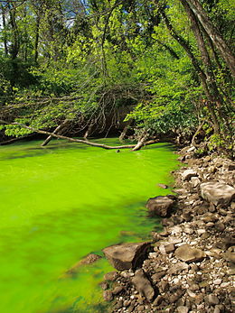
Photo by Alexandr Trubetskoy, CC-BY.
While the trees doubtless consumed some of these liberated nutrients themselves, others were washed away by streams and rivers, ending up in the oceans. Today, agricultural use of phosphorus and nitrogen fertilizers produces a similar kind of nutrient-rich runoff. When it reaches the ocean, this “vitamin soup” jacks up the rate of reproduction of algae; a process called eutrophication. At this point, it all sounds well and good. The issue that makes it deadly enough to cause a mass extinction, though, is that when those supercharged populations of algae die, they die in great numbers. The rotting those billions of dead algae cells consumes all the available oxygen in the water, creating “dead zones” which lack dissolved oxygen. Any fish swimming into such a dead zone must turn around immediately, or asphyxiate. Sadly, this happens regularly today in places like the Gulf of Mexico, where the Mississippi River efficiently delivers nitrogen and phosphorus washed off farm fields in the central United States. Human sewage is another rich source of nutrients; when it enters freshwater lakes or rivers, it can drive this same harmful “boom and bust” cycle that depletes the water of oxygen.
Once the supply of oxygen was exhausted, remaining unrotted dead algae rained down on the seafloor in profusion. Hence: a lot of black (organic-rich) shale. You may have heard of fracking, the process by which humans use high-pressure fluids to shatter organic-rich rocks deep underground, allowing natural gas to flow out. The targets for those fracking operations are mostly Devonian black shales. The Bakken Shale in North Dakota, and the Marcellus Shale in western Pennsylvania are today enticing targets for natural gas exploration because of events that occurred during the late Devonian mass extinction.
Callan Bentley cartoon.
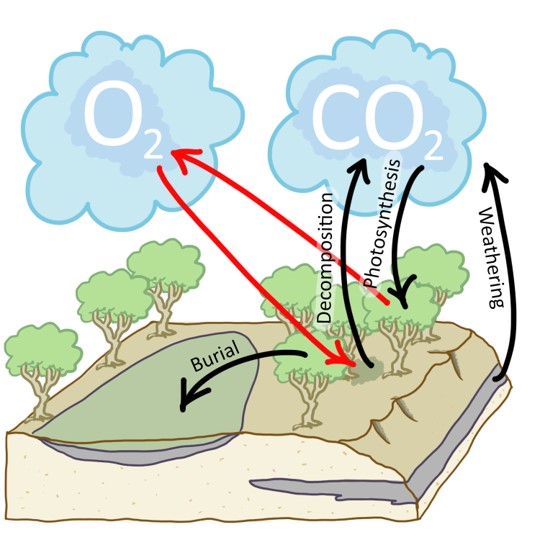
So that is part of the story, but producing thousands of cubic miles of black shale has implications for the planet’s climate, too. Removal of all that organic carbon from the biosphere means that the atmosphere will be relatively depleted in CO2, which is of course a greenhouse gas, helping warm the climate. When CO2 levels are drawn down, there’s less heat retained by the planet, and global cooling can result.
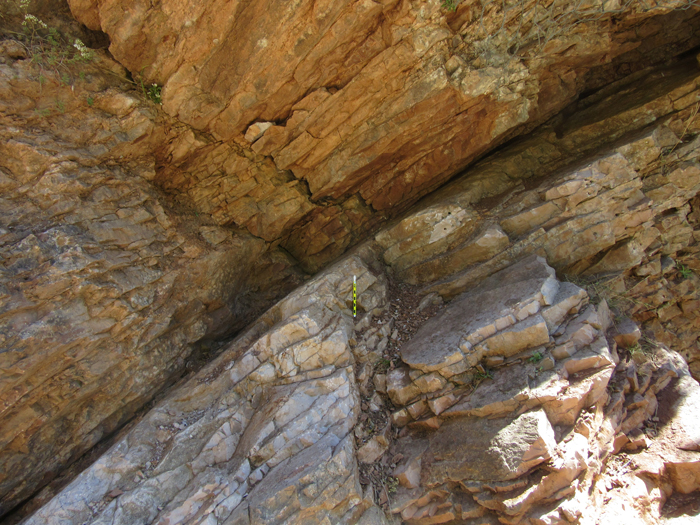
As with the end-Ordovician extinction, there is evidence for a new build-up of glacial ice during the late Devonian. In the Appalachian basin of Maryland, Pennsylvania, and West Virginia, distinctive glaciogenic sedimentary layers can be observed from the late Devonian. Given that paleomagnetic reconstructions put this part of ancestral North America about 30° south of the equator at the time, this implies fairly cold conditions indeed!
As with Snowball Earth, the end-Ordovician glaciation, or the Pleistocene “ice age,” the evidence of glaciation can be seen in faceted, striated clasts, tillites, and dropstones.
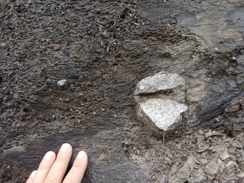
Callan Bentley photo.
From Ettensohn, et al. (2020); reproduced with permission.
Just to bring the discussion of the late Devonian mass extinction full circle, consider anew the black shales laid down on the seafloor, robbing the Devonian atmosphere of its warming CO2. As we extract and burn natural gas from these shales today so that we may produce energy, we *finally* oxidize all that fossil carbon, which had remained sequestered underground for more than 300 million years and would have continued to do so if industrialized humans hadn’t shown up. The CO2-induced warmth that would have saved the Devonian biota from an ice age is now being unleashed on the Holocene (and maybe inducing the Anthropocene…).
End-Permian extinction
Callan Bentley photo.
The end-Permian mass extinction was the most extreme of any in Earth history. It’s sometimes dubbed “The Great Dying,” with 62% of marine genera going extinct, as well as severe impacts among terrestrial biota. Perhaps only 17% of species on Earth survived it. It’s the sharp cliff at the end of the “Paleozoic Plateau.” It’s the closest our biosphere has ever come to being deleted. Writer Peter Brannen astutely called it “the worst thing that ever happened.”
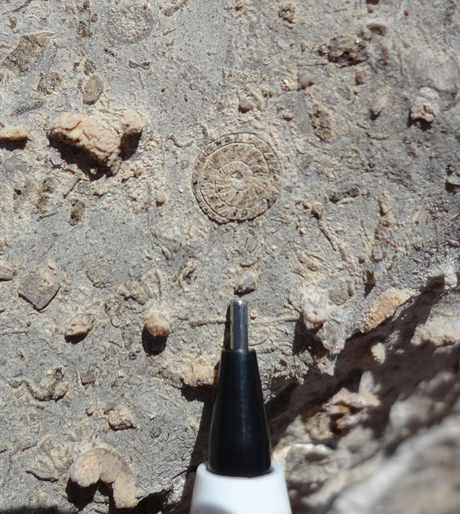
By the end of the Paleozoic, life had rebounded from the late Devonian extinction. In the sea, crinoids and their cousins the blastoids were having a heyday. Tabulate and rugose corals had made great progress in building up reefs in the late Paleozoic ocean, reefs that almost certainly served as shelter and nurseries for many other species, as modern scleractinian coral reefs nurture fish, shrimp, crabs, etc. Giant single-celled fusilinid foraminiferids were rolling around the seafloor like fat grains of rice.

Max Bellomio imagery, via Wikimedia.
On land, the Glossopteris seed fern reigned supreme, at least over the southern supercontinent Gondwana. In its shade, the waterproof amphibian descendants called reptiles had diversified and spread into a great number of ecological roles. Dominant among them were the synapsids, those that used to be dubbed “mammal-like reptiles.” In some cases, these animals could grow to large sizes. You would not have wanted to meet Dimetrodon in a dark alley. The sail-like “fin” rising from its back is its most eye-catching feature, but its mouth was full of sharp teeth.
Also worth noting are the cynodonts, which are probably the direct ancestors of the mammal lineage. Cynodonts were not as large as the therapsids, though, and many of them were hungry. With massive heads bearing powerful jaws and saber-like teeth, Gorgonops and its kin were fearsome beasts. The therapsids had several advantages over their less derived pelycosaur relatives. They had a fully-upright stance, with their limbs always beneath the body. There is also potential evidence that they were endothermic (also called ‘warm-blooded’) and had at least some hair. Many species show ‘whisker pits’ in the skull, which is good bony evidence of hairs that were once anchored in these pits.
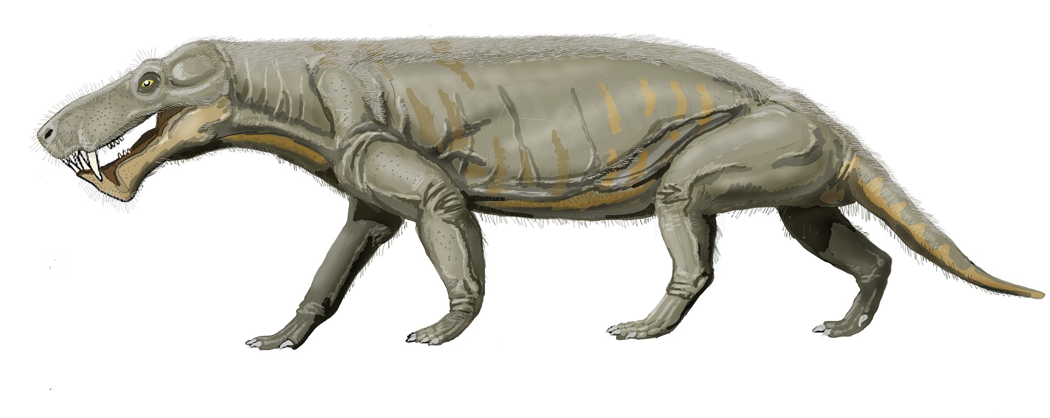
Reconstruction by Dmitry Bogdanov via Wikimedia.
Another group of reptiles had a relatively subdued presence during the Carboniferous and Permian: the sauropsids. These animals included the ancestors of modern lizards, snakes, crocodiles, and birds, as well as the dinosaurs who would dominate the Mesozoic.

Gorgonops and Dimetrodon went extinct at the end of the Permian, along with 2/3 of therapsids. Some cynodonts survived, and these diversified during the Mesozoic that followed, some of them ultimately leading to you and me. One that practically overran the world in the early Triassic was Lystrosaurus, whose populations rose unchecked after the the demise of all its predators. But in the Mesozoic, it was the sauropsids that diversified most successfully, and led to dinosaurs, plesiosaurs, ichthyosaurs, pterosaurs, and mosasaurs. They were the big winners from the end-Permian extinction. But there were so many losers…
NPS photo; public domain.
There were two pulses to the end-Permian extinction. Because they were separated by ~8 million years, it has become commonplace in recent years to hear them discussed independently: the Capitanian (or ‘end-Guadalupian’) at 260 Ma and the true end-Permian event at 252 Ma. Both appear to have the same general cause: global warming.
The careful study of variations in oxygen isotopes in strata spanning the Permian-Triassic boundary shows an lightening of the oxygen content of the oceans. This correlates with a big boost in heat energy, making 18O-based water molecules as likely to evaporate as 16O-based water molecules. Using the ratio of 16O to 18O, it has been calculated that the global ocean warmed by about 6°C. As with the discussion of ‘cooling by 5°C’ in the end-Ordovician extinction above, please realize that it takes a truly enormous amount of energy to shift ocean temperatures by six whole degrees Celsius. That extra energy would have been radiated to space, had it not been trapped by extra CO2 in the late Permian atmosphere.
Now let’s consider where that extra CO2 came from, and then examine the havoc it caused in the ocean.
There were two major large igneous provinces [LINK HERE TO LIP CASE STUDY] that erupted during the late Permian. The first was in China: the Emeishan Traps, where “Traps” derives from the Swedish word trappa, meaning “stairsteps.” This refers to the step-like landscape where the many layers of a vast flood basalt province get etched out. (The Deccan Traps in India have a similar morphology, as do the lava layers of the Columbia Plateau in eastern Washington state.) The Emeishan basalts erupted from 265 to 259 Ma.
Photo by Александр Лещёнок, CC-BY via Wikimedia.
The second, much larger, was in Siberia. Today we call it the Siberian Traps. The Siberian Traps represents one of the biggest eruptive episodes in Earth history. Presumably the result of a mantle plume slamming into the bottom of the north Asian continent, the volcanic rocks of the Siberian Traps have been shown to span the Permian-Triassic boundary, including the mass extinction at 252 Ma.
From a video by the USGS.
Size estimates of the Siberian Traps boggle the mind: A volume of more than 1.5 million cubic kilometers of lava was erupted, smothering roughly 2 million square kilometers of northern Siberia. That is enough basaltic lava to bury the entire contiguous United States to a depth of half a mile. It’s enough basalt to make three towers, each with a footprint of 1 square kilometer, that reach to the Moon.
So much lava being erupted carries with it a commensurate amount of volcanic gas. Most of that gas is water vapor, which is rapidly removed from the atmosphere via precipitation. But the second most common volcanic gas is CO2, and you know what that does.
Not only that, but one of the layers that the Siberian Traps basalt passed through on its way from the mantle to the surface was a vast Carboniferous-aged coal field (the world’s largest) in the Tunguska Basin, which caught fire and burned, adding even more CO2 to the total that was released! Estimates are that the level of CO2 in the atmosphere reached to at least 3000 ppm, and maybe as high as 30,000 ppm. Average estimates for the end-Permian are ~8000 ppm. (For reference, in 2022, the world was at about 420 ppm, up from ~280 ppm in pre-Industrial times.) So the end of the Permian had twenty times as much CO2 in its atmosphere as we do today, an insane level that would have warmed the planet to an astonishing degree.

Photo by Yukio Isozaki; reproduced with permission.
A warm climate doesn’t necessarily spell the end of the world, but in this case, the oceans played a key role. In the modern world, with cold polar regions and warm tropics, our ocean vigorously circulates in a vast, floppy loop. The energy that drives this flow of water comes from the difference in temperature (and thus density) of the water. When warm water grows cold, it gets more dense, and it sinks. Sinking water pulls other water after it, and a flow is induced. But in the Permian, as the polar oceans warmed up to roughly the same temperatures as the tropics, this flow was reduced, and — apparently — stymied completely. In short, the oceans became stagnant.
As with the late Devonian, this produced anoxia in the oceans, which is recorded as usual by jet black sedimentary deposits. The anoxia was at first most pronounced in the deep ocean, but it appears to have eventually invaded the coastal shallows. This is where most marine life makes its home, and that was of course quite disastrous.
Worse, though, is what happened when the Sun’s rays hit the anoxic shallow water. This is the rare combination of factors that promotes the growth of sulfur-reducing bacteria, which release hydrogen sulfide gas (H2S) as a waste product. You know H2S: it’s the stink of rotten eggs — or the nauseating stench of really gross farts. In low levels, it’s revolting and annoying, but in high levels, it’s deadly. The appearance in seafloor sediments of little raspberry-shaped clusters of pyrite (FeS2) suggest that the ocean at the end of the Permian was quite rich in sulfur. The inference is that these distinctive purple bacteria must have bloomed in profusion without any of their usual microbial competitors.

J. Glass photo; permission requested.
Thus the oceans were not only anoxic, but also probably also euxinic — the word that describes being thoroughly infused with H2S. In 2005, Lee Kump and colleagues suggested something bold – that the oceans were so euxinic during the end-Permian that H2S began to exsolve out of the sea and into the air, where it acted like an agent of chemical warfare, gassing terrestrial animals to death.
Another potential “kill mechanism” that applies to terrestrial species has its roots in a layer of rock salt that the Siberian Traps eruption also pierced, exploded, and scattered as it erupted. The chemicals that were released are thought to be the sort that destroy ozone (O3), which humans have done using the famous chlorofluorocarbons (CFCs) that were banned by the Montreal Protocol. If the stratosphere’s ozone layer was severely damaged at the end of the Permian, that would have increased the flux of ultraviolet light (particularly UV-B) to the surface of the planet. This deadly radiation would have potentially driven up rates of mutations and cancers for any organism that was exposed to it (i.e., only those who lived on land).
Modified from a photo by Toedi3614, via Wikimedia.
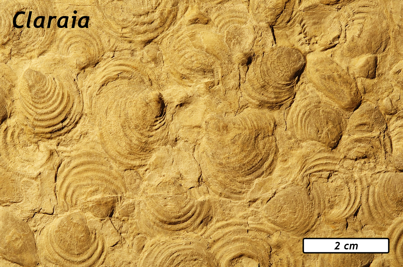
In the aftermath, the world lay obliterated, an apocalyptical denuding of the biosphere that probably reeked of rotten eggs. On land, the formerly terrifying forms of Dimetrodon and Gorgonops lay still; corpses rotting away in the foul air. The forests of sphenopsids and lycopsids were done forever. From the rotting foliage, a few therapsids nosed out and sniffed the air. In the sea, there were no more blastoids, no more fusulinid forams, no more trilobites or rugose corals. No more eurypterids; no more goniatitic ammonoids. Brachiopods were greatly reduced in number and diversity (a 96% decline). They would be replaced by the bivalves in the years to come. Still depleted in oxygen and utterly emptied out, the early Triassic seas were overtaken by one genus of clam that was adapted to low-oxygen conditions. Claraia spread far and wide, unimpeded by any competition. It’s so omnipresent and numerous that as a monoculture, it makes an excellent index fossil for the first part of the Triassic period: a bizarro “Clamworld.”
This was the one big reset of Earth’s biosphere –phyla that had dominated the oceans for 200 million years were gone, and oceans would never look the same. The survivors went on to diversify into the Modern Fauna; mollusks would now reign supreme, scleractinian corals would build reefs, and echinoids, sea stars and sea cucumbers would now represent the echinoderms (replacing crinoids and blastoids).
End-Triassic extinction
Photo by Anita Gould, CC-BY, via Flickr.
Therapsids flourished in the Triassic, now that their synapsid competitors had been suffocated. These crocodilian relatives were attended by the first dinosaurs, but dinosaurs were the sideshow rather than the main act. Only after the end-Triassic extinction could the dinosaurs surge forward and dominate the Mesozoic land surface. But first, their crocodilian overlords must be cleared away.
In the sea, about half of the Triassic genera didn’t make it into the Jurassic. Almost every kind of ammonoid and bivalve was decimated. Ammonoids had evolved a ceratitic morphology, which is an index fossil for the Triassic. Also in the seas were a menagerie of marine reptiles, many of whom were snuffed out by the end-Triassic extinction event. Walrus-like reptiles called placodonts and the seal-like nothosaurs totally perished, while some of their ichthyosaur and plesiosaur cousins eked a way through, and would re-diversify in the Jurassic and Cretaceous.
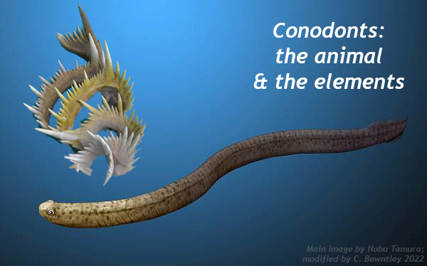
Photo illustration by C. Bentley (2022), using the background illustration by Nobu Tamura and element photo by Wikipek, both CC-BY, and both via Wikimedia.
One small animal of note, the conodonts (a kind of thin, eel-like jawless fish) had been a fixture of Earth’s oceans from the Cambrian onward. They were practically as common in the oceans as water molecules, and left their jaws and gill support structures behind as an uniquely valuable index fossil. But the end-Triassic got them, too. Their long run on Earth came to an abrupt end at 202 Ma.
Now that you know who died and who survived, let’s examine the “why?”
Like the end-Permian crisis that preceded the Triassic, the mass extinction that brought it to an end appears to be a case of (1) “large volcanic province erupts,” (2) “CO2 levels spike,” and (3) “global warming ensues.” In this case, a hot spot is not to blame.
Williamborg image, after Blackburn (2013), via Wikimedia.
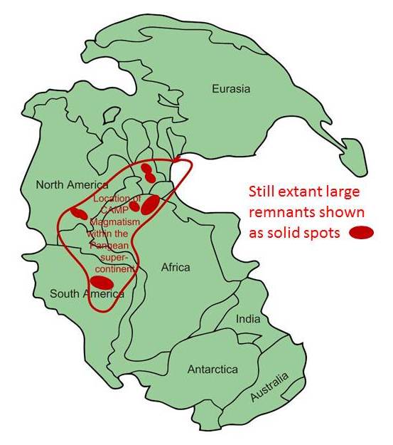
Instead, it was the titanic breakup of the most gargantuan supercontinent ever. As rifting split Pangaea and opened the spindly Atlantic Ocean down its center, the underlying crust was thinned dramatically. In what is today eastern North America, a series of rift basins — the Newark Supergroup basins — opened up along normal-faulted hinges, dropping down like trap doors. These basins did an excellent job catching immature sediment from the surrounding highlands, but they also released the pressure on the hot mantle beneath, which partially melted and made its way upward along the fault system. What issued forth was an enormous amount of basaltic magma. And it wasn’t only in North America; huge quantities of basalt and gabbro were produced in adjacent regions of northeastern South America, northwestern Africa, and southwestern Europe. Though its various major volcanic centers have now been separated by seafloor spreading of the Atlantic Ocean, they were once adjacent. Today we call it all the Central Atlantic Magmatic Province (CAMP).
Ultimately, CAMP may have erupted even more basalt than the Siberian Traps, but a good amount of it has since weathered away. Its total volume is estimated at something between 2 and 3 million cubic kilometers of mafic igneous rock. CAMP rocks cover 11 million square kilometers. The eruptions came in four major pulses over the span of about 600,000 years. That’s a lot of magma making it to the surface (and degassing CO2) in a relatively short amount of time.
Modified from a public domain image via Wikimedia.
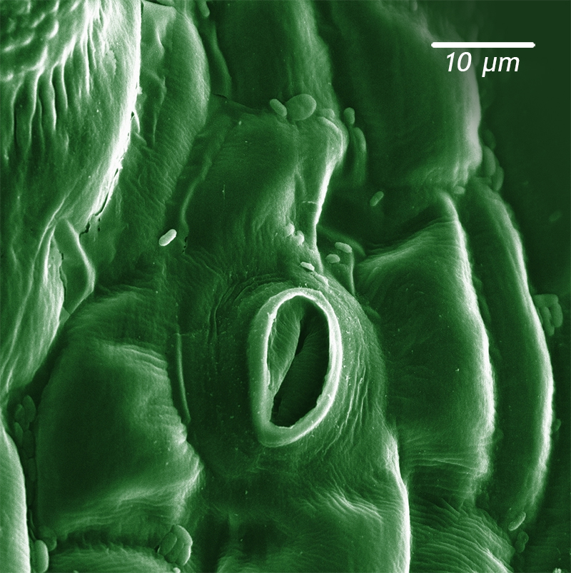
An interesting study about the Triassic extinction uses plant fossils [LINK TO FOSSIL PLANT CASE STUDY] as a proxy for examining CO2 levels at the time. On the underside of plant leaves are little holes that allow gas exchange with the atmosphere. These holes, called stomata (singular: stoma), are like little doors that let CO2 in to enable photosynthesis and waste O2 out after glucose has been made. In modern plants, the number of stomata inversely correlates with atmospheric CO2 levels. The higher the CO2 level, the fewer stomata are needed to get what the plant needs. Under conditions of lower CO2, plants require more stomata to let in sufficient air to extract the same absolute amount of CO2. So simply by collecting fossil leaves and counting their stomata with a microscope, we can arrive at a sense of how CO2 levels varied across the Triassic/Jurassic transition. Jennifer McElwain and colleagues (1999) analyzed fossil leaves from end-Triassic strata in Greenland and Sweden. They found that the stomata density decreased dramatically at the end-Triassic, commensurate with an atmospheric CO2 level that was seven or eight times as high as we have today. That means a 3-4°C jump in temperature, above and beyond temperatures that were already ~3°C warmer than today’s. [If you’re interested in this technique, the Smithsonian has a citizen science project for counting stomata that you can help out with.]
With the planet’s biota reset once again, it was finally time for the dinosaurs to have their day.
End-Cretaceous extinction
Dinosaurs came in two major groups, the saurischians and the ornithischians. With the crocodile-like Triassic therapsids now mostly dead, the dinosaurs diversified and persisted for tens of millions of years. They dominated terrestrial ecosystems in a pervasive and enduring fashion. Other reptiles colonized the air (pterosaurs, and eventually birds too) and the sea (plesiosaurs, ichthyosaurs, huge turtles like Archelon, and eventually mosasaurs too). Giant reptiles were everywhere during the Jurassic and Cretaceous. The world was their oyster.
Callan Bentley photo.
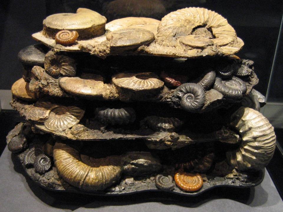
Speaking of oysters, the sea had plenty of those during the middle and late Mesozoic. Some of them encrusted the shells of clams called inoceramids that had shells a meter in diameter. Another bizarre bivalve group was the rudists, which resembled Sesame Street’s Oscar the Grouch in their trashcan-like morphology. Swimming among them were spiral-shelled cephalopods: the ammonitic ammonoids, which bore distinctly fractal-looking suture patterns between segments of their shells. They make for superb index fossils for the Jurassic and Cretaceous. But along with the dinosaurs and other giant reptiles, their time on Earth came to an end on one very bad day.
Before we get to that day, there are several items that need mentioning. First off, the Cretaceous was hot in general, all around the world. There is no evidence of glacial ice anywhere on the planet during this “hothouse” climate. This, combined with a vigorous rate of seafloor spreading, pushed oceans up onto the continents. In North America, this allowed the Western Interior Seaway to develop as the Sevier Orogeny produced an adjacent foreland basin.
Photograph by Nichap, CC-BY, via Wikimedia.
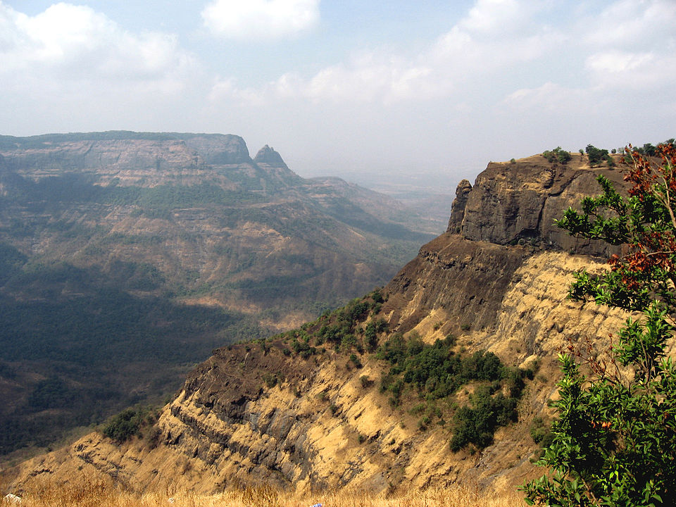
Then things started going wrong. The first, you’ll be shocked to hear, was the eruption of another large igneous province. This one was in western India: the Deccan Traps. As with the Emeishan Traps and the Siberian Traps discussed above, this is a landscape of step-like mesas and plateaus, as a thick stack of basalt flows has been dissected by more recent streams. Like them, it is astoundingly large: 1 million cubic kilometers of basalt, slathering half a million square kilometers of western India (it may have originally been much higher in volume and area, but as with CAMP, it looks like much has been eaten away by subsequent erosion). The eruptions were relatively rapid – from beginning to end, it may have lasted only 30,000 years. At the time of its eruption, India was its own small continent, surrounded by the Indian Ocean — i.e., this was prior to its collision with southern Eurasia. It is inferred that the eruptions were triggered by the island continent’s drift over the Réunion hotspot, a long-lived welt in the Earth’s mantle that is still producing lava today, at namesake Réunion Island itself.
Callan Bentley photo.
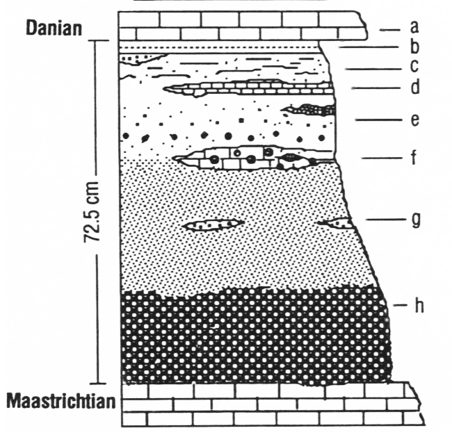
Up until 1980, that alone would have been viewed as entirely sufficient to explain the end-Cretaceous (a.k.a. “K/T” or “K/Pg”) extinction. But in 1980, a son/father team published a paradigm-shifting paper in the journal Science that dredged up the specter of catastrophism anew. Walter Alvarez and his father Luis Alvarez, with others, published a bombshell of a paper that laid out the case for an extraterrestrial impact as the cause of the end-Cretaceous extinction. The younger Alvarez was working as a geologist in the central range of mountains that run down the spine of Italy, the Apennines. He studied the stratigraphy of the limestones and shales there, and one day got to wondering about the nature of the boundary between the Cretaceous and the Tertiary*. He noticed that it really came down to a single layer of clay between two ~4 cm thick limestone strata. He had a really great outcrop in Bottaccione Gorge, a canyon near the town of Gubbio. Below this horizon, Alvarez saw distinctive Cretaceous radiolarian fossils. Above it, none.
* When Alvarez did this work, “Tertiary” was still used as a period by the International Commission on Stratigraphy. Only more recently (2003) did “Paleogene” replace it.

Graph redrawn by C. Bentley (2022)
It occurred to him to wonder how much time was packed into that clay layer. Was it 10,000 years, or 100,000, or something else? His father, a Nobel-prize-winning physicist, suggested examining the clay layer from the perspective of the small but (presumed-) constant flux of micrometeorites to Earth. Luis Alvarez advised his son to look for something distinct to outer space sources, that would have built up gradually, and thus could be used to calibrate how much time had elapsed while the clay was deposited. The elder Alvarez suggested the element iridium, which (he hypothesized) should have a more or less constant flux to Earth’s surface.
But the amount of iridium they actually measured were out of this world. Literally.
There was so much iridium packed into that clay layer that the Alvarez team found another hypothesis more likely: this had to be fallout from a single giant meteorite impact somewhere else in the world.
Though many geologists initially were skeptical of this “catastrophe” of a hypothesis, they soon got busy testing it, by checking the Cretaceous/Paleogene (K/Pg) boundary elsewhere in the world, to see if other locations also shared this iridium anomaly. Sure enough: they showed the iridium anomaly, too! In addition, they started documenting additional evidence of an impact: (1) spherules and (2) shocked quartz.
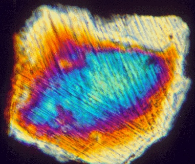
Photograph by Glen A. Izett, USGS, public domain.
Spherules are little glass droplets that form when rock, melted instantaneously by the tremendous heat of the impact, is flung into the air as billions of tiny droplets. These cool and solidify before they rain out onto the landscape: little glass beads that speak of unimaginable violence. Shocked quartz is a little bit different: it starts off as a solid crystal of the common mineral quartz, but then it deforms as the powerful shock wave of the impact passes through it, wrecking its previously precise crystal lattice but not destroying the integrity of the grain by melting or disintegrating it. These distinctive features were first identified in the aftermath of nuclear bomb testing, and were decisively associated with extraterrestrial impacts by the legendary Gene Shoemaker, the “grandfather of impact geology.”
The K/Pg boundary layer thickened toward the Americas, and toward the Gulf of Mexico even more. In their search for oil and gas deposits, the Mexican state petroleum company, Pemex, had mapped a vast circular structure that was mostly under the Gulf of Mexico, but also had about a third of its area lapping over onto the thumb-like Yucatán Peninsula. At first, it was inferred to be a big, extinct volcano, but in 1981, geophysicists Glen Penfield and Antonio Camargo suggested it was an impact crater instead, and indeed that it was the one responsible for the end-Cretaceous extinction. One reporter, Carlos Byars, wrote up the announcement for the Houston Chronicle. Somehow, almost no one noticed.
Luckily, a decade later, Byars was covering a geology conference where the crater’s location was still an enigma. In an astonishing moment, the journalist Byars let the scientists in on what to him must have seemed like “old news” — and now the geological community had found its ground zero, its Big Kahuna.
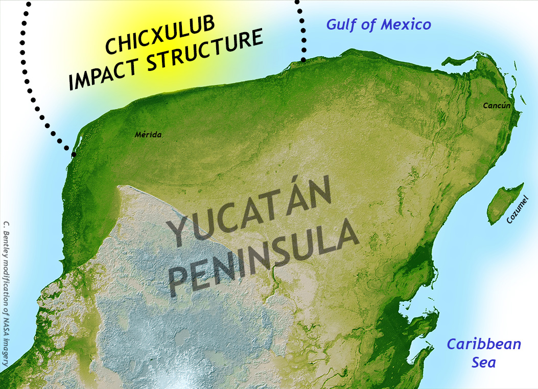
C. Bentley annotation of a NASA image.
The crater was centered on a small port town called Chicxulub. Thus, the structure has come to be known by that name. The structure is about 180 kilometers (110 miles) in diameter and 20 kilometers (12 miles) deep, but it is now mostly hidden from view underneath the subsequent 65 million years worth of sedimentation – limestone, mostly. These overlying limestones have slumped downward a bit over the course of the Cenozoic, allowing a distinctive ring-shaped scarp to develop in the overlying limestone of the Yucatán. All along this ring are water-filled sinkholes, called cenotes. The entire arc of cenotes is a candidate World Heritage Site, not only for its relevance to the end-Cretaceous extinction, but also because the great pre-Columbian civilization of the Mayans utilized these cenotes for access to water.
Impact experts can model the size of the impacting object (a meteorite or a comet, or more agnostically named, a bolide) by the size of the crater it leaves behind. In this case, the impactor would have been about ten kilometers across, roughly the diameter of San Francisco, or Mount Everest. The energy released would have been something on the order of 100 million megatons of TNT. If you’ve seen footage of the Chelyabinsk meteorite’s detonation in 2013 over Russia, you’ve seen what half a megaton looks like. Just multiply that by 200,000,000.
Recently, Robert DePalma and colleagues (including Walter Alvarez and Jan Smit) published a new site they call “Tanis” in North Dakota. It exposes strata of the Hell Creek Formation. Though the Hell Creek is a widespread regional geological unit, Tanis holds an incredible concentration of fossils that appear to have been deposited within hours of the impact. There are many superlative features of Tanis, but one of the most evocative is the presence of meteorite impact evidence inside the organisms fossilized. Specifically, fish breathe with gills, and those gills strain oxygen from the water. At Tanis, about half of the fish fossils have impact spherules caught in their gills, suggesting they were alive and breathing as impact debris was raining down upon their waterway. This astounding details suggests an amazing level of precision for the date of the Tanis deposits – they literally show the very last day of the Cretaceous period.
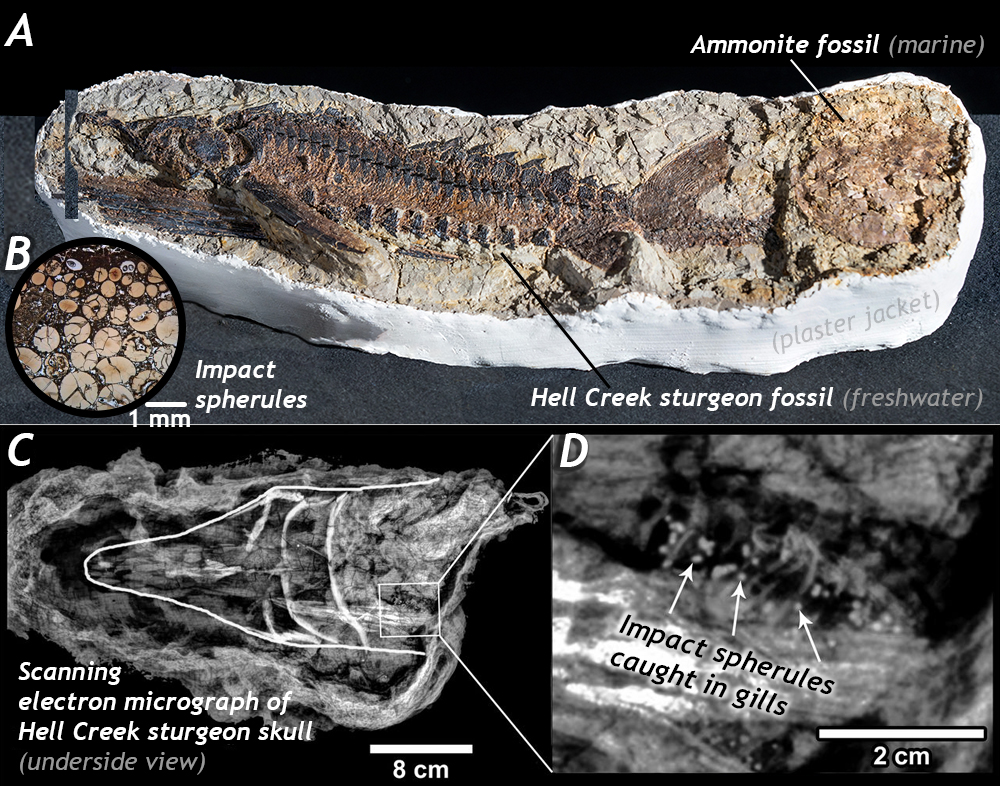
Images B, C, and D are from Figures 4 and 6 of DePalma, et al. (2019).
So there is now substantial evidence for a major extraterrestrial impact at the very, very end of the Cretaceous. But how did that kill half of life on Earth? Various kill mechanisms have been proposed, including from the radiative heat of the impact, blunt force trauma from its shockwave, subsequent forest fires, violent tsunamis, ocean acidification, and finally a prolonged “nuclear winter” from small particles suspended in the stratosphere. Upending the food chain, some or all of these traumas destabilized the biosphere and ended the Mesozoic Era. What followed was the Age of Mammals, the Cenozoic — the time that would ultimately lead to us.
It’s worth noting that dinosaurs aren’t all gone… birds are with us today, and like mammals and plants (particularly angiosperms), the birds have undergone adaptive radiations to lead to the familiar ecosystems we see across the modern Earth.
Other ‘mass’ extinctions
Peter Brannen’s excellent book The Ends of the World recaps the Big Five, but also looks in detail at numerous other mass extinction events, including some in the Precambrian and some that have yet to occur (i.e., in Earth’s future). A few notable examples outside the traditional Big Five are briefly described below:
The Great Oxidation “Event”
Callan Bentley photo
Mass extinctions are relatively easy to detect when the organisms dying (and replacing them) leave behind body fossils with hard parts. The picture is much more difficult to discern when all organisms were microscopic. In the early Proterozoic Eon, Earth transitioned from an oxygen-free atmosphere to one with a decent amount of free oxygen (O2). Though this is called the Great Oxidation “Event,” [GOE] it is not a very sudden event at all. Traditionally, it is viewed as the span from 2.4 Ga to 2.0 Ga: that’s 400 million years, a very drawn-out “event.” Other names include the Oxygen Crisis, the Oxygen Catastrophe, and the Oxygen Revolution, each of which puts its own spin on interpreting the rise of this important gas.
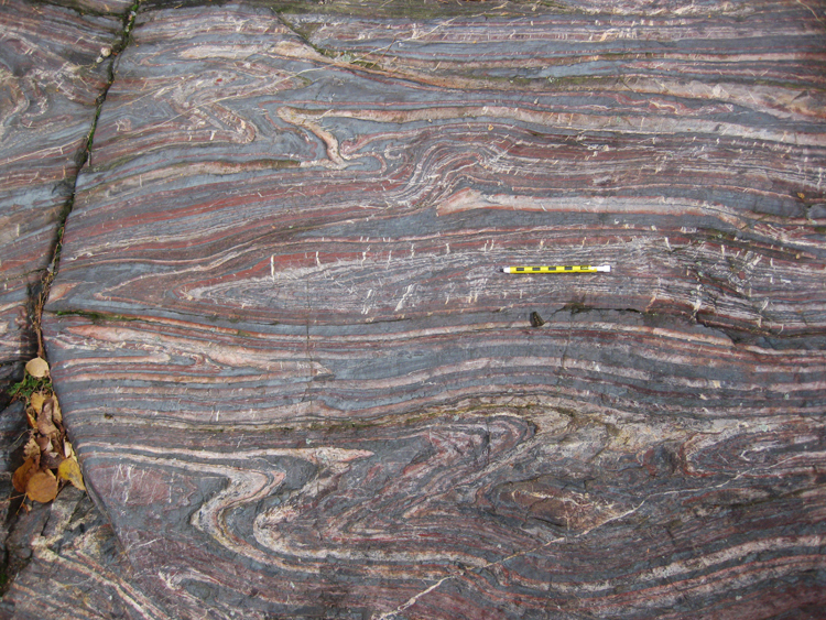
Prior to the GOE, the planet’s atmosphere lacked significant free oxygen. We know this because of unusual chemical sedimentary rocks that could only form in an ocean that is largely oxygen free (banded iron formations [BIFs]), as well as grains of minerals like pyrite and uraninite in clastic sedimentary rocks. These signatures of the absence of oxidizing conditions imply a very different early Earth.
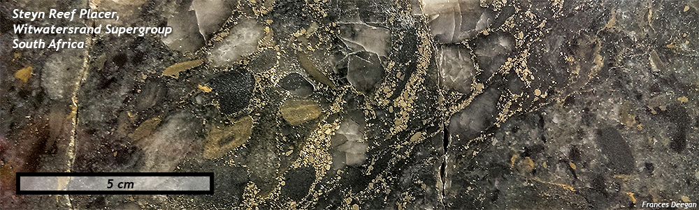
Photo by Frances Deegan; reproduced with permission.
Those anoxic conditions are preserved in Archean strata and those of the early Proterozoic. But by the middle of the Proterozoic, the BIFs and detrital pyrites peter out, and we see the first appearance of oxidized terrestrial sediments (red beds). These are river and floodplain sediments deposited in contact with copious oxygen – enough O2 to rust their iron content through and through.
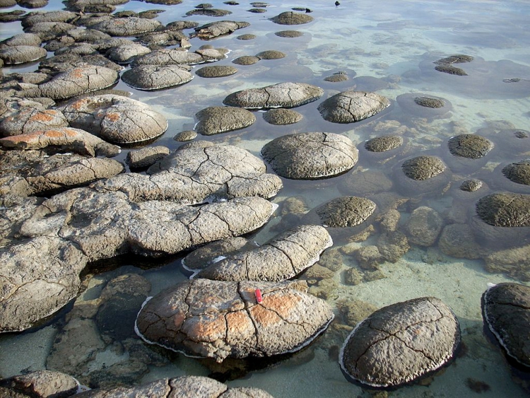
Photo by Alicejmichel via Wikimedia
So where did all this free oxygen come from, and what was the impact on the biosphere? Oxygen is a waste product of photosynthesis, so any photosynthetic organism produces it in proportion to the amount of glucose it generates. Of particular note are cyanobacteria, which are preserved from Archean and younger times as stromatolites. Long before true plants evolved, photosynthetic cyanobacteria was busy for billions of years pumping oxygen out into the oceans (and thence by diffusion into the atmosphere).
This oxygen, being the highly reactive element it is, immediately reacted with whatever was suitable and available: carbon, for instance, making CO2. Or silicon, making SiO2. Or maybe iron dissolved in the seawater; that would oxidize and settle out as magnetite or hematite. But the rates of production matter: if oxygen was being churned out at a rate greater than the availability of these other reactive elements to buffer its rise, then it eventually began to accumulate in the atmosphere, available for reactions, but finding insufficient reactive elements to bond with. It built up and built up.
But while life was chemically fine for cyanobacteria, surrounded by their waste. Sulfur-reducing bacteria, for instance (the ones implicated above in end-Permian euxinia) cannot survive in the presence of free oxygen; it’s a deadly poison to them. They are not alone: many groups of microbes cannot tolerate free oxygen. Some persist today in isolated low-oxygen settings such as swamp muck, but many others probably went extinct as the GOE took hold. How many exactly, and what were their characteristics? We’ll never know: microbes just don’t fossilize with the level of detail we would need to answer those questions. It seems reasonable to infer it was a great many, but we must become comfortable with the uncertainty about the specifics.
The Cambrian explosion
Creative Commons Attribution-Share Alike 4.0 International license.
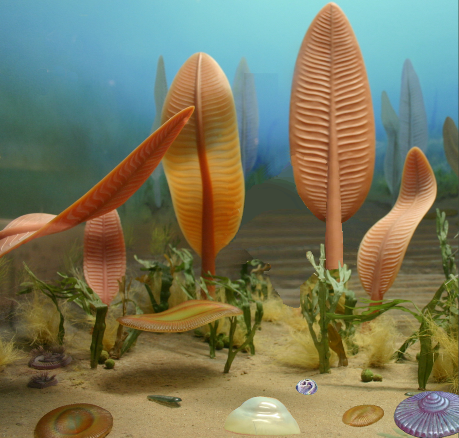
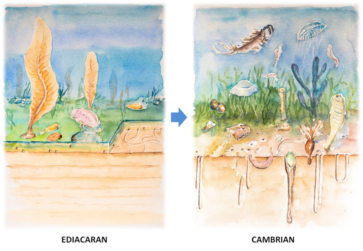
The Cambrian Explosion is justifiably celebrated as a great blossoming of diverse animal life forms, well recorded in the geologic record by their profusion of shells and other hard parts. But it was preceded by a time when soft bodied, sessile animals were widespread across the globe. These were the Ediacaran biota, a diverse group of organisms presumed to be animals. Some resembled jellyfish, and others looked similar to modern sea pens. Some might have been the ancestors of mollusks. But the suddenness of the Cambrian Explosion implies that it was an adaptive radiation, and therefore took place in an ecological space that had recently been cleared out of its previous inhabitants. The Ediacara had no chance against their Cambrian competitors, not only because they lacked armor, but also because the Cambrian critters destroyed their ecosystem.
The Ediacaran period was a time of microbial mat-dominated ecospace, apparently with very few organisms exploiting higher levels in the water column, nor were there any burrowing very deeply into the sedimentary substrate below. The lack of bioturbation in Ediacaran sediments suggests it was a “sealing” ecosystem, largely anchored to the sediment/water interface, and rarely deviating from it.
Watercolor painting by Richard Bligny for an article by Jean Vannier; inspired by an original in Fedonkin et al. 2007.

C. Bentley annotation of Martin Smith photo via Wikimedia.
Once vascular body plans and hard parts had evolved, however, the diverse animals of the Cambrian were freed from being bound to the bottom of the sea. Some swam high above, such as the fearsome predator Anomalocaris, while many others burrowed into the sediment below. The latter group includes inarticulate brachiopods and various worms. These organisms dug into the sediment, using its bulk as protections against predation. In so doing, they churned up the sediment, disturbing the continuity of the bedding. This bioturbation is a “trace fossil” signal of the Cambrian Explosion. Indeed, the very oldest beds of the Cambrian are defined by the first appearance of the trace fossil Treptichnus pedum. (These burrows are presumed to be the probing burrows of priapulid worms, which continue to make similar traces today.)
By all means, celebrate the glories of the Cambrian Explosion, but spare a thought for the poor, doomed Ediacara that came before!
Eocene-Oligocene transition
Modified by CB from a NASA public domain image.
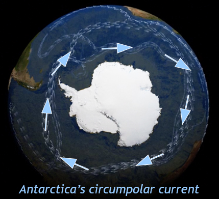
Halfway through the Cenozoic Era, Earth’s climate shifted into a cooler state. The most obvious cause for this cooling was the separation of Antarctica from southern Australia and southern South America. This divergence opened up a swath of open ocean that encircled Antarctica on all sides. A new ocean circulation pattern developed, the circum-polar current, which wrapped around Antarctica like a doughnut. These endlessly orbiting waters cooled and cooled, isolating Antarctica from the rest of the world. In as little time as 100,000 years, deep sea ocean temperatures dropped globally by 4°-5°C. By 30 Ma, there were new glaciers growing on the southern continent.
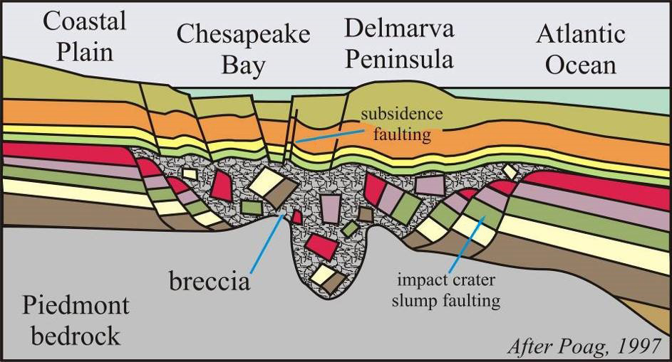
Callan Bentley cartoon (2003) after Wylie Poag original (1997).
Another series of events that may be relevant are at least three substantial bolide impacts in the northern hemisphere: Popigai in Siberia (35.7 ± 0.2 Ma), Toms Canyon offshore from New Jersey (~35 Ma), and Chesapeake Bay, Virginia (35.5 ± 0.3 Ma). As mentioned in the discussion of the end-Cretaceous impact, dust and debris may be thrown up to the stratosphere by an impact. Suspended in this rain-free portion of the atmosphere, the particles can screen out a portion of incoming solar radiation, reducing global temperatures.
Art by Heinrich Harder (1858-1935), public domain via Wikimedia.
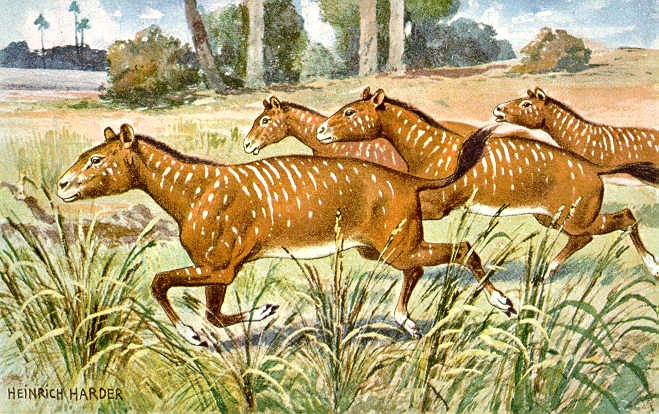
This shift in the climate resulting in a turnover of organisms, both in the sea and on the land. In the oceans, spiky foraminiferida were replaced by forms with less surface area. Bivalves adapted to warm conditions died out, replaced by more cold-adapted species. On land, grasslands increased, taking over land previously covered by forest. Mammals living on land had to adapt to these cooler, drier conditions – and we see a transition from browsers (that eat leaves off bushes and trees) to grazers (that “mow” the grass) at this time. Horses, rhinos, camels, and antelopes all spread at this time.
Pleistocene megafauna
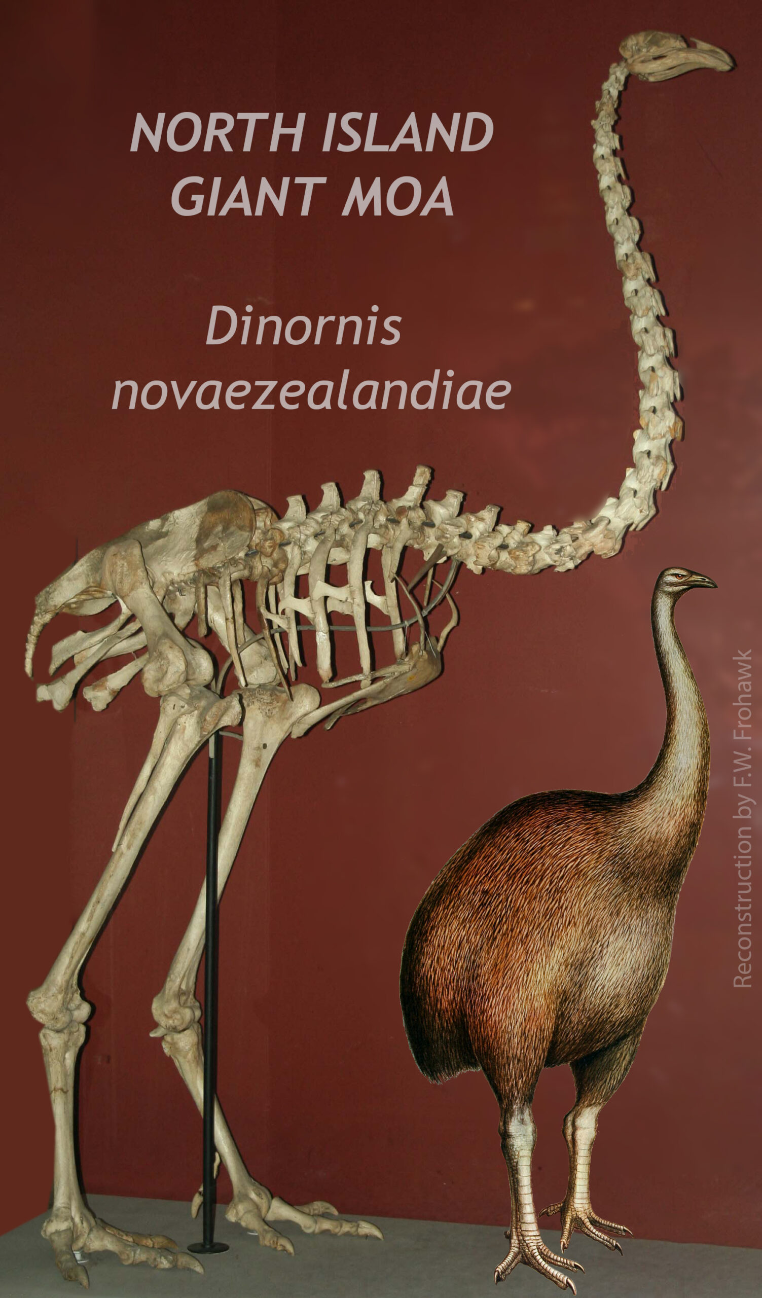
Photo mashup of public domain imagery from Wikipedia.
.jpg)
Unlike the preceding examples, the most recent mass extinction skipped sea life, skipped plant life, skipped small mammals, and skipped nocturnal animals. It just focused on large mammals and birds. The dead include giant ground sloths, mammoths and mastodons, glyptodonts, huge bears, saber-toothed cats of several varieties, and (in Australia) marsupial equivalents of many of these. There were even vultures of unusual size, who presumably fed on the corpses of these great beasts. These last presumably enjoyed a great glut for a short while, and then saw their smorgasbord go bare. Other huge birds included the phorusrhacids, the elephant bird, and the moas.
Various causes have been proposed for the extinction of these “megafauna,” from a new ice age to a meteorite impact. The ice age hypothesis is particularly weak, however, since the most recent Pleistocene glacial advance was just one in a series of dozens that stretch back in time to ~2.6 Ma. Why these animals did fine for the first several dozen but succumbed only at the most recent one is not explained. Evidence for a meteorite impact has been documented in recent years, but while it corresponds in timing with the North American extinction of the megafauna, it post-dates the Australian extinction event, and pre-dates the Madagascar extinction event.
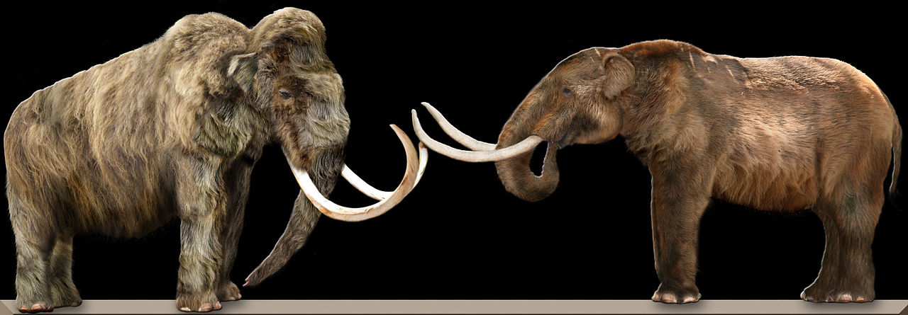
Image by Dantheman9758, CC-BY, via Wikimedia.
Diagram by ElinWhitneySmith (2006), after Martin (1989), public domain via Wikimedia.
Key to understanding the Pleistocene megafauna extinctions is the fact that the timing for the extinctions varied from continent to continent. Further, it seems to be strongly tied to the arrival of the first humans to arrive there. It happened earliest in Australia (~45,000 years ago), and most recently in the Americas (14,000 to 13,000 years ago), and more recently still in isolated islands, such as Madagascar or New Zealand. The Pleistocene “overkill” hypothesis (first articulated by Paul Martin) links the predatory habits of our own species with the loss of these giant beasts. This explanation is controversial, as some people see it as unfairly maligning indigenous people around the world.
The one place where the Pleistocene megafauna extinctions happened least was the one place where the megafauna had hundreds of thousands of years to get used to Homo sapiens: Africa. Africa is famous today for its surviving megafauna: elephants, hippos, rhinos, lions, and giraffes are the sizes and sorts of animals that used to be found on the other continents, too. This is a classic example of the adage “the exception that proves the rule” — where “the rule” is that when humans arrived in a place that was home to animals with no natural fear of humans, the humans rapidly killed the animals. Africa is “the exception,” as this is humanity’s birthplace, and the animals there have evolved in tandem with humans, developing a healthy aversion to them.
The modern biodiversity crisis
Right now, you and I may be living through another mass extinction, one brought on by humans’ severe impact on the natural world. Dubbed “the Sixth Extinction” to denote its severity as approaching the Big Five, the modern biodiversity crisis is harder to get a handle on, since we are in the middle of it. The tools we use to assess mass extinctions recorded in the deep time record of rocks don’t work for the present. So this is a trickier comparison to make. But there is a strong case that humanity’s influence has been both geological in scale and negative in effect. Some geoscientists have teamed up with environmental activists to suggest that we should consider the current moment as a new, distinct geologic epoch, the Anthropocene.
Elizabeth Kolbert’s Pulitzer-prize-winning book The Sixth Extinction is a well-written account of the various relevant factors. Uniquely among books about the current environmental crisis, it is exceptionally well grounded in the geological context. She notes numerous factors that contribute to the modern crisis:
-
- Habitat destruction and fragmentation
- Invasive species
- Disease
- Pollution
- Climate change
Rates of extinction documented in the modern day (using extant species and a historical timeframe) match or even exceed rates calculated from fossil turnover during the Big Five mass extinctions. However, these accelerated rates have only been operating for a geologically brief amount of time (a few centuries). The numbers are alarming, but it’s not an ideal scientific contrast, since all the confounding variables haven’t been controlled for. It’s comparing “apples to oranges.” That said, what other choice do we have? Humans cannot help the fact that they live in the present.
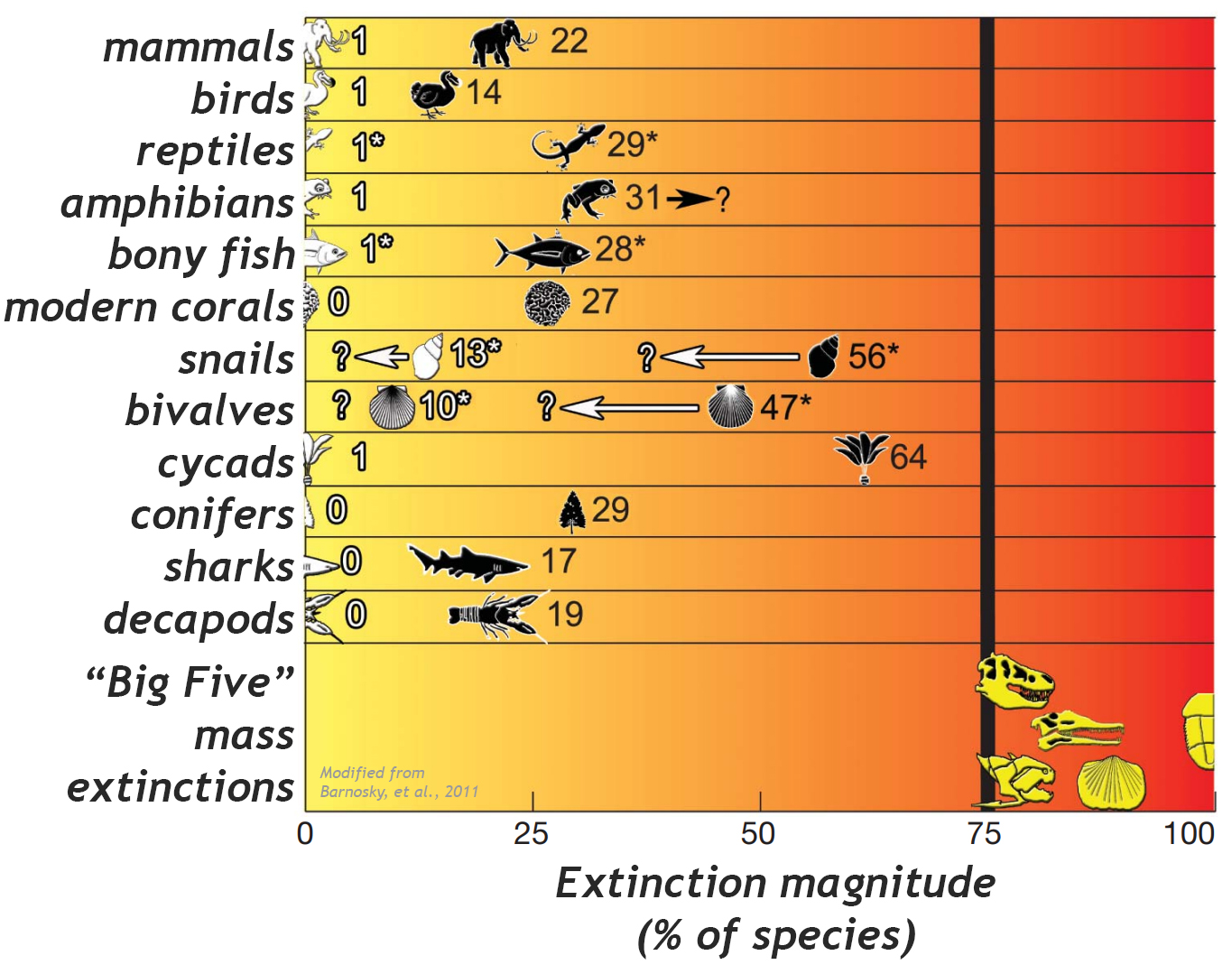
high as 43%.
In an attempt to assess the actual levels of extinction that have so far occurred and can reasonably be “blamed” on humanity, Barnosky et al. (2011) don’t actually find very many. They examined species documented by the main international body the focuses on conservation biology, the IUCN. (This is the group that maintains the “red list” of endangered species.) How many of those species have gone extinct in the past 500 years? How does that compare with extinction rates determined from fossils in stratified rocks at each of the “Big Five?” Thankfully, they show that there is a pretty big discrepancy between modern numbers and ancient numbers. But the question of time hangs over this comparison – 500 years is almost nothing in the geological sense of time. It is hard to compare a modern rate of 1 species per 500 years with an ancient rate of 75% of all species per 100,000 years. The timescales are too radically discrepant.
If the modern rates play out for another 500 years (or 1000), will they cross the threshold of being a mass extinction? If the answer is yes, and we wait until then to decide it’s actually a big problem, then it would be too late. Asking the question now allows us to take action to prevent a sixth mass extinction from becoming a reality.
The last life on Earth
C. Bentley modification of an original by Oona Räisänen, via Wikimedia.
Far in the future, perhaps 2.5 billion years from now (maybe sooner), life on Earth will cease. This will be the final mass extinction our planet is capable of pulling off. Two sets of processes need to be considered, those of Earth’s interior and those of our star, the Sun. Plate tectonics is responsible for continuously revitalizing Earth’s surface, but it is driven by heat from the planet’s interior. Heat production is maintained through time by radioactive decay of unstable parent isotopes, such as 40K, 232Th, 87Rb, and 238U. But there are fewer and fewer of these isotopes every day. Our planet is cooling off, and eventually it may get too cool to maintain plate motions. Estimates of this sad date put it about 1.45 billion years in our future. A cooler core means less liquid outer core through time, as the solid inner core grows larger. Eventually, when the core becomes completely solid, the magnetic geodynamo of the outer core will cease, and our planet will lose its atmosphere-protecting magnetic field. This exposes the atmosphere (and the surface hydrosphere) to erosion by the solar wind. Life won’t last much longer in those conditions – Earth would increasingly come to resemble Mars.
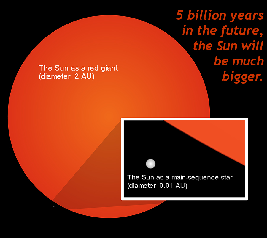
Regardless of these “local” details, the fate of our planet ultimately hinges on the future the Sun. The Sun is a G-type star, and those grow in volume through time as they burn through their hydrogen fuel. Ironically, as they lose mass, they swell up to a larger size. Less mass means less gravity holding them in a tight, dense ball; older stars have relaxed and stretched out into space.
In our solar system, that will mean that Mercury and Venus are likely fated to be consumed by the Sun as it expands outward. Earth’s location is likely about where the surface of the Sun will reach in ~5 billion years when it becomes a elderly red giant, but a reduction in the Sun’s mass also means a reduction in the Sun’s gravitational hold on Earth, and so the planet will likely shift into a more distal orbit, further out from where we currently orbit. Nonetheless, the larger, closer Sun will fry the Earth, evaporating away its oceans and sterilizing its surface.
Franck, et al. (2006) made estimates of how Earth’s temperature will respond to this swollen star, and compared these estimates of its future temperature to the tolerances seen in modern examples of various domains and phyla. Multicellular life is estimated to have 800 million years left, according to that study, or possibly up to 1.2 billion years, while single-celled eukaryotes will last longer, perhaps 1.3 to 1.5 billion more years. Prokaryotes are hardiest of all at high temperatures; it is thought they will persist until about 1.6 billion years from now.
And that will just about do it for life on Earth.
Summary
To recap these mass extinctions, here is a summary table, in chronological order:
| Name | Date | % extinct* (taxonomic loss) |
Putative cause |
| Great Oxygenation Event | 2.4-2.0 Ga | ¯\_(ツ)_/¯ | Cyanobacterial pollution of the atmosphere |
| Cambrian Explosion | ~539 Ma | all the Ediacara | Hard parts arms race |
| Late Ordovician | ~445 Ma | 52% | Global cooling |
| Late Devonian | ~372 Ma | 40% | Excessive carbon burial due to the advent of trees + global cooling |
| End-Permian | 260-252 Ma | 83% | Ocean anoxia induced by eruption of the Siberian Traps |
| End-Triassic | 201 Ma | 73% | Global warming induced by the eruption of CAMP |
| End-Cretaceous | 66 Ma | 40% | Meteorite impact ± Deccan Traps |
| Eocene-Oligocene | 34 Ma | 15% | Global cooling |
| Pleistocene | 18-10 ka | (just megafauna) | Human overhunting |
| The end of all life on Earth | 1.6 billion years in the future (?) | 100% | Sun expanding & overheating the planet |
* Most numerical estimates from McGhee, et al. (2013).
Further reading
Luis W. Alvarez, Walter Alvarez, Frank Asaro, and Helen V. Michel, 1980. “Extraterrestrial cause for the Cretaceous-Tertiary extinction,” Science 208, p.1095–1108.
Anthony D. Barnosky, Nicholas Matzke, Susumu Tomiya, Guin Wogan, Brian Swartz, Tiago Quental, Charles Marshall, Jenny L. McGuire, Emily L. Lindsey, Kaitlin C. Maguire, Ben Mersey, and Elizabeth A. Ferrer, 2011. “Has the Earth’s sixth mass extinction already arrived?” Nature 471, p.51-57. DOI:10.1038/nature09678
D.J. Beerling and D.L. Boyer, 2002. “Reading a CO2 signal from fossil stomata,” New Phytologist 153, No. 3, p. 387-397.
Callan Bentley, 2012. “Permian fusulinid forams from west Texas,” Mountain Beltway blog post.
Terrence J. Blackburn, Paul E. Olsen, Samuel A. Bowring, Noah M. McLean, Dennis V. Kent, John Puffer, Greg McHone, Troy Rasbury, and Mohammed Et-Touhami, 2013. “Zircon U-Pb Geochronology Links the End-Triassic Extinction with the Central Atlantic Magmatic Province,” Science 340 (6135): p.941–945. doi:10.1126/science.1234204.
Peter Brannen, 2017. The Ends of the World. Ecco, 336 pages.
Robert A. DePalma, Jan Smit, David A. Burnham, Klaudia Kuiper, Phillip L. Manning, Anton Oleinik, Peter Larson, Florentin J. Maurrasse, Johan Vellekoop, Mark A. Richards, Loren Gurche, and Walter Alvarez, 2019. “A seismically induced onshore surge deposit at the KPg boundary, North Dakota,” Proceedings of the National Academy of Science 116 (17) p.8190-8199. https://doi.org/10.1073/pnas.1817407116
Frank R. Ettensohn; D. Clay Seckinger; Cortland F. Eble; Geoff Clayton; Jun Li; Gustavo A. Martins; Bailee N. Hodelka; Edward L. Lo; Felicia R. Harris; Noushin Taghizadeh, 2020. “Age and tectonic significance of diamictites at the Devonian–Mississippian transition in the central Appalachian Basin,” in Geology Field Trips in and around the U.S. Capital, edited by Christopher S. Swezey and Mark W. Carter. Geological Society of America, Volume 57. https://doi.org/10.1130/2020.0057(04)
M.A. Fedonkin, J.G. Gehling, Grey K., G. Narbonne, and P. Vickers-Rich, 2007. The Rise of Animals. The Johns Hopkins University Press, Baltimore. 325 pp.
Seth Finnegan, Kristen Bergmann, John M. Eiler, Jones, D.S., David A. Fike, Ian Eisenman, Nigel C. Hughes, Aradhna K. Tripati, and Woodward W. Fischer, 2011, “The magnitude and duration of Late Ordovician-Early Silurian glaciation,” Science 331, p.903–906.
S. Franck, C. Bounama, W. von Bloh, 2006. “Causes and timing of future biosphere extinctions,” Biogeosciences, European Geosciences Union, 3 (1), p.85-92.
Tony Hallam, 2004. Catastrophes and Lesser Calamities: The causes of mass extinctions. Oxford University Press, 226 pages.
Elizabeth Kolbert, 2014. The Sixth Extinction. Henry Holt and company, 319 pages.
Mandy Hofmann & Ulf Linnemann, 2013. “The Late Ordovician (Hirnantian) Lederschiefer Forma- tion in Thuringia – evidences for a glaciomarine origin from the Berga Antiform (Saxo-Thuringian Zone),” Geologica Saxonica 59. p.133-139.
Lee R. Kump, Alexander Pavlov, Michael A. Arthur, 2005. “Massive release of hydrogen sulfide to the surface ocean and atmosphere during intervals of oceanic anoxia,” Geology 33 (5): p.397–400. https://doi.org/10.1130/G21295.1
Florentin. J-M. R. Maurrasse and Gautam Sen, 1991. “Impacts, Tsunamis, and the Haitian Cretaceous-Tertiary Boundary Layer,” Science 252 (5013):1690-3 DOI:10.1126/science.252.5013.1690
Jennifer C. McElwain, D. J. Beerling; F. I. Woodward, 1999. “Fossil Plants and Global Warming at the Triassic–Jurassic Boundary,” Science 285 (.5m, Peter M. Sheehan, David J. Bottjer, and Mary L. Droser, 2013. “A new ecological-severity ranking of major Phanerozoic biodiversity crises,” Palaeogeography, Palaeoclimatology, Palaeoecology 370: p.260–270. https://doi.org/10.1016/j.palaeo.2012.12.019
Douglas Preston, 2019. “The Day the Dinosaurs Died,” The New Yorker, April 8 issue.
David Raup, 1992. Extinction: Bad Genes or Bad Luck? Norton, 210 pages.
Jack Sepkoski, 2002. “A compendium of fossil marine animal genera”. Bulletins of American Paleontology 363: p.1–560. Ithaca, NY: Paleontological Research Institution.
Jan Smit; Alessandro Montanari; Nicola H.M. Swinburne; Walter Alvarez; Alan R. Hildebrand; Stanley V. Margolis; Philippe Claeys; William Lowrie; Frank Asaro, 1992. “Tektite-bearing, deep-water clastic unit at the Cretaceous-Tertiary boundary in northeastern Mexico,” Geology 20, p.99–103 (1992).
Laura Soul and Rich Barclay, 2017. “Can You Help Us Clear The Fossil Air?” Smithsonian Magazine blog post.
Steve Stanley, 2016. “Estimates of the magnitudes of major marine mass extinctions in earth history,” Proceedings of the National Academy of Sciences. 113 (42): E6325–E6334. doi:10.1073/pnas.1613094113.
Peter Ward, 2008. Under a Green Sky. Harper Perennial, 256 pages.
___________________