Quaternary Quandaries: Defining the Geologic Now

KEY CONCEPTS:

At the end of this chapter, students should be able to:

• Describe how geoscientists define start and end dates for periods on the geologic time scale.
• Differentiate between the different epochs and ages within the Quaternary Period.
• Differentiate between the different ages within the Holocene Epoch.
• Describe how recent changes to the Holocene were made.
• Discuss the significance of the Meghalayan Age and its associated GSSP.
• Explain the current debate and discussions surrounding the potential defining of a new Anthropocene Epoch.
• Identify what a GSSP, or “Golden Spike” is in the geologic record.

How do we define the time in which we live? Can it be done in a word or an idea? Or, is it through the sum of our material past, the objects we leave behind to tell our story? Do we get to define our time, or is it something left to those who follow us later on?

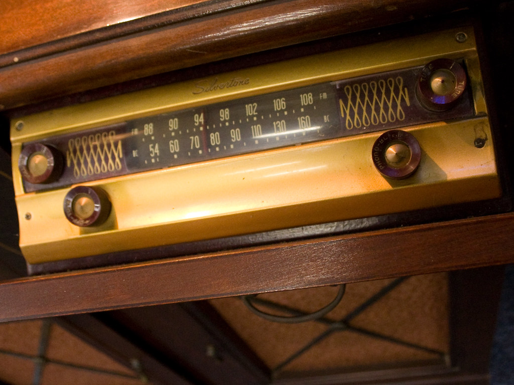
The band of time can be modeled metaphorically using the old AM/FM radios you may have seen a car, the kind with knobs you can use to tune it. Radio tuners have a starting frequency and ending frequency which, in the case of the FM band, runs from 87.5 to 108 MHz. If you wish to find a particular station, or frequency, all you needed to do was turn the dial. Each frequency was already defined, depending upon your location, by a given radio station. If you wanted the rock station, you tuned it to perhaps 100.7 MHz, and so on. Because it was already there and defined before you used it, you knew what to expect and what the parameters of a particular location on that radio dial was like. Radio stations are not really boundaries in the FM spectrum, but metaphorically they can be viewed as little waystations, locations of significance, amidst the staticky stuff in between, with nothing of distinction to set it apart from any other position on the spectrum.

Geologic time is very similar. How can we use it to give some kind of meaning to the expanse of time?

The Geologic Time Scale is a model that has been developed by lots of people working over lots of time. Their work that helps us answer these difficult questions. As is the case with all models, the Geologic Time Scale is wrong in many ways. However, it is still very useful. As time and knowledge accumulate, we improve the model. Such improvements can include everything from simple date changes to larger-scale changes like the introduction of new periods or epochs. However change progresses, the time scale is a model that represents our best understanding of the band expanse of time as we understand it. The geologic time scale is not static, but dynamic. It is managed by the International Commission on Stratigraphy (ICS), an affiliate of the International Geological Union. The work of the ICS is to compile ongoing research into the various portions of the time scale in order to refine the boundaries of the Eons, Eras, Periods, and Epochs we use to define time. To do this, Global Stratotype Sections and Points (GSSPs) are identified that provide a consensus marker in time for any given boundary. These GSSPs are often referred to as “Golden Spikes”, a reference to the golden spike used to complete the Trans-Continental Railroad, as they serve as clearly-defined time markers that allow researchers (and professors and students!) to share in common discussion.

But, how hard is it exactly to define such boundaries in time?

Over the course of this case study, we will explore three critical questions:

1. 1. How do we use the geologic time scale as a model to make sense of time?
   2. How do we make changes to this model as we learn more about time?
   3. Can we use this model to help us define our own time in the present and recent past?

The geoscientists working with the Subcommission on Quaternary Geology are wrestling with these questions. Their subcommission is a part of the International Commission on Stratigraphy (ICS). Ultimately, this case study will explore a proposed new epoch, the Anthropocene Epoch. Before we get there, we need to spend some time exploring how the ICS has gone about defining our most recent era, periods, epochs, and ages. Hopefully, we can then revisit the above questions and have some satisfying answers.

A Quaternary Quandary

Our modern geologic periods, epochs, and ages have been a state of flux. Currently, we live in the Meghalayan Age of the Holocene Epoch of the Quaternary Period of the Cenozoic Era of the Phanerozoic Eon. However, there have been many changes to this hierarchy over the last few hundred years, with significant changes recently.

Our modern sense of geologic time began in northern Italy. In 1759, a man by the name of Giovanni Arduino introduced three terms to help make sense of the geology of the Alps where he worked. He used the term “Primary” for the ancient metamorphic cores of the mountains, “Secondary” for the hard sedimentary rocks on the flanks, and “Tertiary” for the sedimentary rocks in the foothills, which were not quite as hard. Primary and Secondary were eventually dropped by scientists because they did not always describe what was seen in regions in other areas. Tertiary remained. In 1829, French geologist Jules Desnoyers added the term “Quaternary” to describe the most recent geological materials, including lava flows and loose sediments. The terms Tertiary and Quaternary are still with us, though embattled in different ways, their dates and how they are viewed having changed over time. As recently as 2000, these two periods comprised the entire Cenozoic Era, with the Tertiary Period lasting from 65 Ma until 2.58 Ma and the Quaternary Period running from 2.58 Ma to the present.

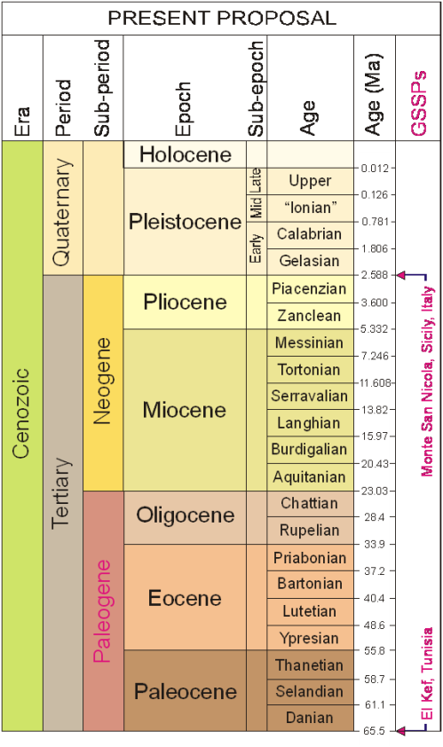
In 2004, the keepers of geologic time, the ICS (International Commission on Stratigraphy) completely dropped the terms Tertiary and Quaternary from the time scale, replacing them with two divisions, the Paleogene Period (66 Ma to 23 Ma) and the Neogene  Period (23 Ma to 2.58 Ma). This was done in order to standardize the Cenozoic Era time periods to be consistent with the rest of the time scale. Marine geologists felt that the Neogene should also encompass all of the most recent portions of time. A major disagreement arose, however, because terrestrial geologists felt that the most recent geological materials on land required that the old term Quaternary Period be retained. These sediments and formations included all of the ice age materials, which are different from Neogene materials prior to 2.58 Ma. Terrestrial workers won the argument and in 2009, the ICS voted to reinstate the Quaternary Period.

The base of the the Quaternary is marked by the beginning of what is known as the Gelasian Stage. The lower boundary of this chronostratigraphic unit is marked by a GSSP location near Gela, Italy, and is primarily a magnetostratigraphic boundary, but secondarily marks the extinction of a number of calcareous nanofossils. Perhaps most importantly, the Gelasian Age (“Stage” is a chronostratigraphic term equivalent to the lithostratigraphic term “Age”) marks the start of the growth of northern hemisphere glaciers and ice sheets. You may know this time by another name: the Pleistocene Epoch. Perhaps images of mammoth, mastodon, saber-toothed cats, and early humans perhaps just popped into your mind!

Currently, the Quaternary Period is broken up into two Epochs, the Pleistocene Epoch (2.58 Ma to 11.7 Ka) and the Holocene Epoch. There is a move to add another time division, something perhaps called “Anthropocene,” but it is not finalized yet. We will come back to that later.

Marine Isotopic Stages: Defining the Pleistocene and Holocene Epochs

The Quaternary Period differs from the Paleogene and Neogene Periods because it is defined by ice age cycles, known as greenhouse (interglacial) and icehouse (glacial) periods. An entire glacial/interglacial cycle typically lasts about 100,000 years and is driven by Milankovitch orbital changes. And, there are enough of these that the record is quite complicated. When you look at the climate record of the Pleistocene Epoch, however, you see many, many more up and down swings in temperature. These smaller, or shorter, changes in temperature during a glacial period are “stadials” and “interstadials”.

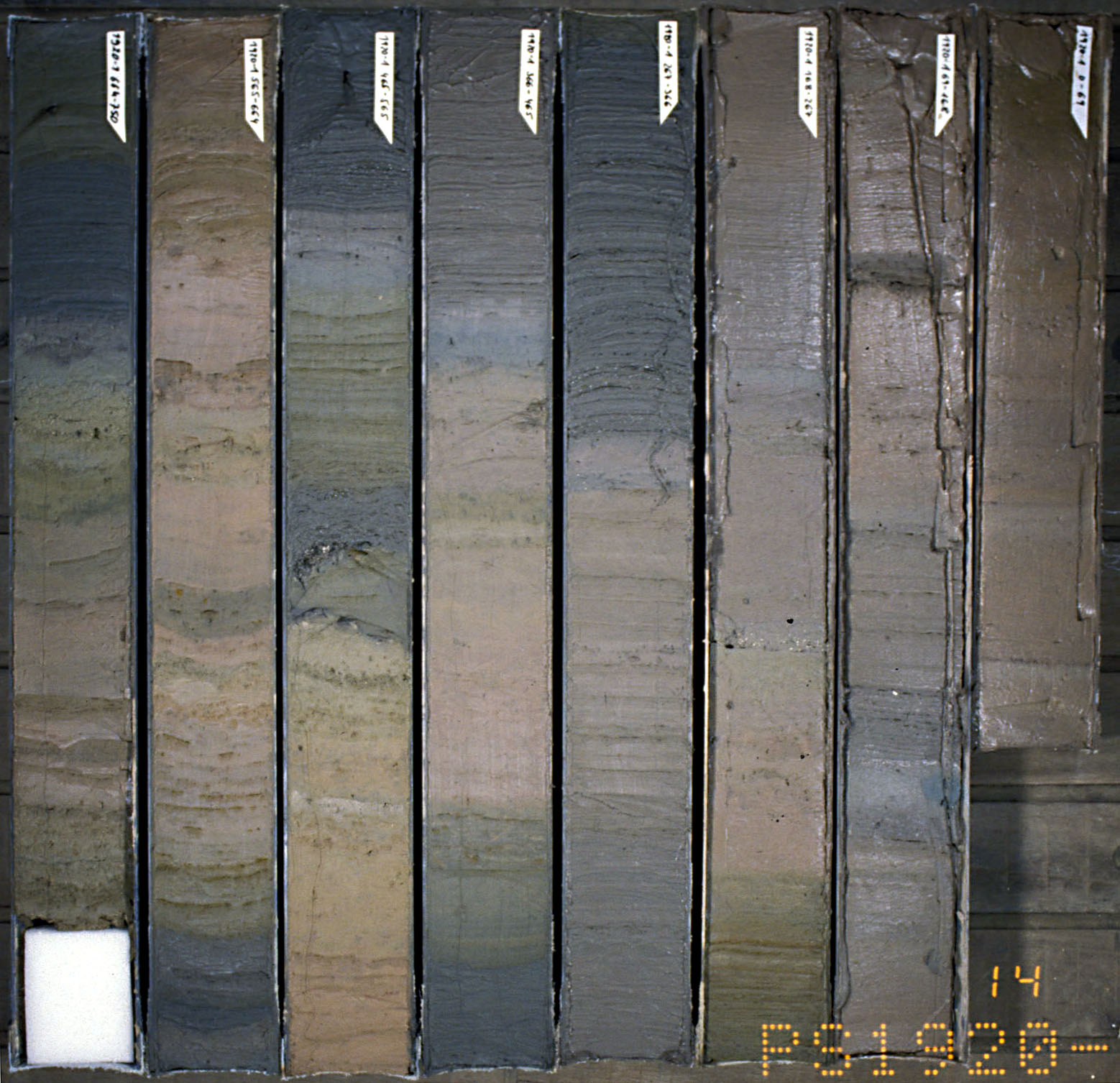
In addition to ice cores, researchers have collected extensive deep sea sediment cores from off the coast of places like Greenland. These sediment cores record critical data, oxygen isotopes in particular. From these, a very fine record of oxygen isotope fluctuations is recorded, which in turn reflect periods of warming and cooling. These alternating periods are called Marine Isotopic Stages (MIS). These stages are numbered from the start of the Holocene Epoch and going backward in time. Even numbers were assigned to cool periods (stadials) and odd numbers to warm periods (interstadials). For example, our current Holocene Epoch was given the number MIS-1, since it is an interstadial warm period. The last major 100,000 year long glacial period, the Wisconsinan (so called in North America), encompasses several isotopic stages, MIS-2,3, and 4.

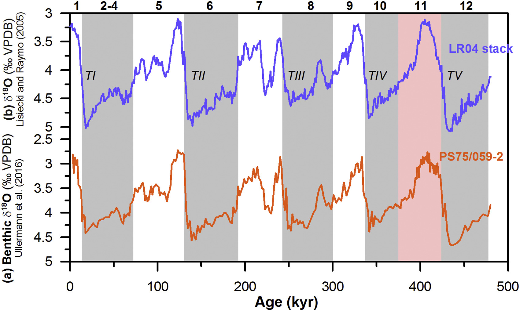
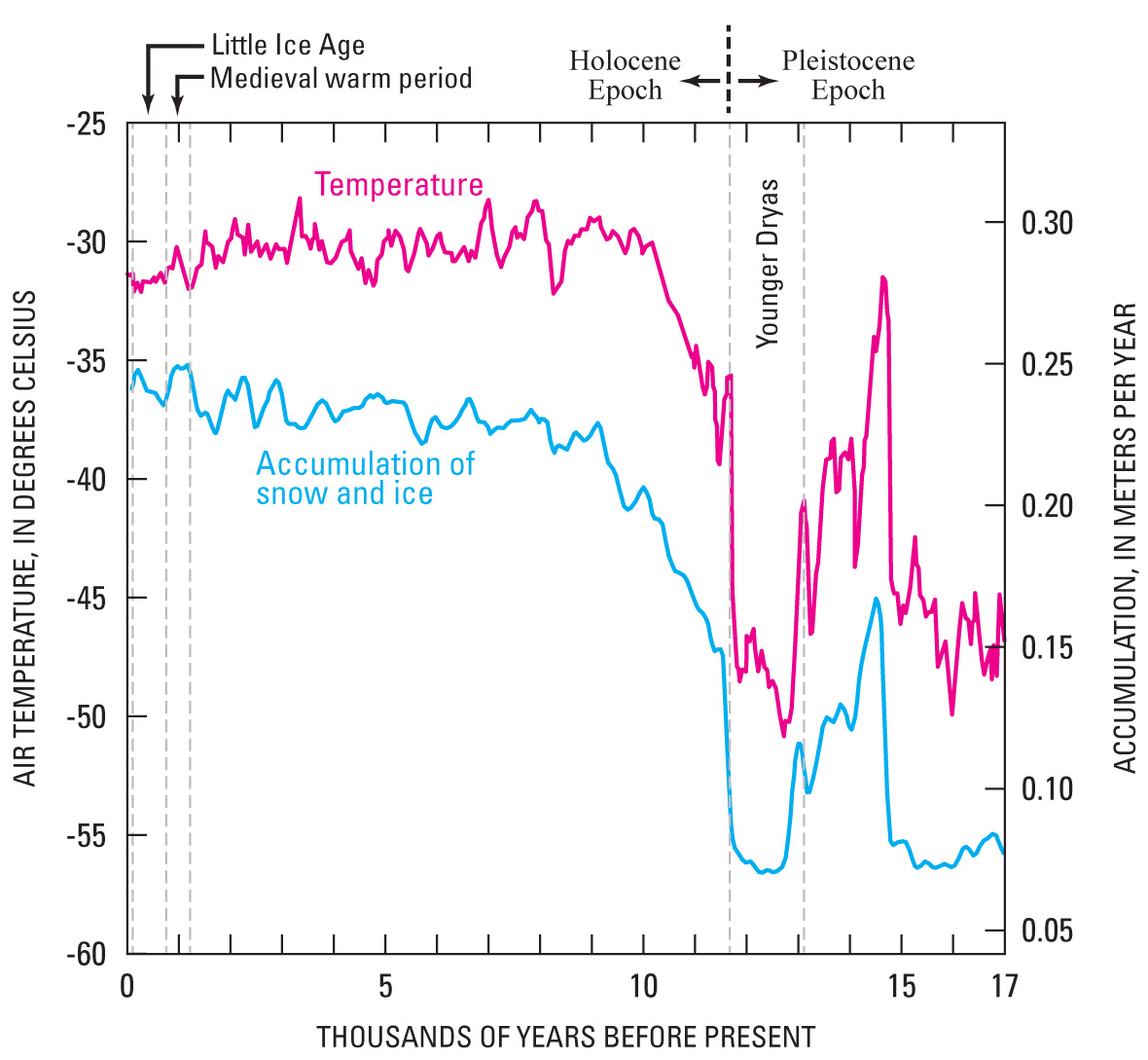
In all, over 100 Marine Isotopic Stages have been identified. These record 2.6 million years of climatic change throughout the Pleistocene and Holocene Epochs. It is worth asking why the Holocene, as MIS-1, is separated out as somehow different from the rest of the marine isotopic stages of the Pleistocene. In short, Holocene climatic records indicate that this interstadial period has not only now exceeded the average length of these (~1000 years) at 11,700 years, but it has also seen a much more stable temperature throughout. This is different than past interstadials during the Pleistocene. Coupled with an aberrant climatic shift at its start called the “Younger Dryas” (discussed later in the chapter), these attributes make the Holocene fairly unique from the Pleistocene.

Today, the Cenozoic Era consists of three well-defined and agreed upon periods, the Paleogene Period, Neogene Period, and Quaternary Period. Defining time is clearly challenging and requires detailed high-quality data. Now that we have firmly established the three Periods of the Cenozoic Era, we need to dive more deeply into the Quaternary Period to explore its epochs…and to see the changes that have been and are afoot there.

What’s in an epoch?

Geologic eons are broken up into eras and eras into periods. Geologic periods are broken up into epochs and epochs into ages. During the Cenozoic Era, the Paleogene Period is broken up into the Paleocene, Eocene, and Oligocene Epochs. The Neogene Period is broken up into the Miocene and Pliocene Epochs. Each one of these earlier Epochs is marked by important evolutionary and geologic changes that define these bands of time. The final Period of the Cenozoic, the Quaternary, is divided up into two epochs, the Pleistocene Epoch and the Holocene Epoch. These are all lithostratigraphic terms, defined by sedimentary rock layers. In terms of time, or chronostratigraphic nomenclature, the rock layers that define an epoch are referred to as a series.

The Pleistocene Epoch

The Pleistocene is an epoch of wicked climatic seesaws. At times, there is a layer of ice a mile thick over southern Canada. At other times, there is nearly nothing of that left. We also tend to define the Pleistocene by its fauna, including mammoths, mastodons, saber-toothed cats, and more. The name Pleistocene comes from the Greek and means “most new,” a term given it by Charles Lyell, back in the 19th century. As mentioned above, the base of the Pleistocene is marked by the start of the Gelasian Age, a time when large ice sheets began to grow in higher latitudes around the world. Based upon there being 40 marine isotope stages identified during this time, there were likely at least 20 glacial cycles during this age. The age ends at 1.8 Ma with the extinction of the nannofossil Discoaster brouweri.

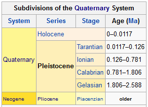
The story of the Pleistocene continues stratigraphically upward into the Calabrian Age (1.8 Ma to 0.774 Ma) into the Chibanian Age (0.774 Ma to 0.129 Ma) and finally to the “Upper” Age (proposed “Tarantian Age,” 0.129 Ma to 0.0117 Ma). The boundary between the Calabrian and Chibanian is marked by the Earth’s last magnetic reversal, but the boundary between the Chibanian and “Upper” Age is marked by the onset of the Eemian interglacial, which is the last warm period before the onset of the Holocene Epoch. Currently the “Upper” Age of the Pleistocene is under consideration for a new name, the Tarantian Age. However, as of just a few years ago from the time of this writing (June 2020), neither a lower or upper GSSP had been defined. In 2018, the upper boundary of a potential Tarantian Age was defined by the onset of the Greenlandian Age of the Holocene Epoch, as defined by a layer within a core taken from the Greenland ice sheet by the Greenland Ice Core Project. The very top of the Tarantian Age occurs at the end of a brief return to icehouse conditions after a significant warm up. This event is referred to as a the “Younger Dryas” and its end is the beginning of the Holocene Epoch and the Greenlandian Age.

This all may seem complicated, full of funny names and obscure dates. There is truth to this on the surface. However, when you peel away all of this complexity, we have described a model that does something conceptually simple: the geologic time scale helps us define time through the environmental change. The model is useful because it is so adaptable.

A Clima(c)tic sidebar – The Younger Dryas

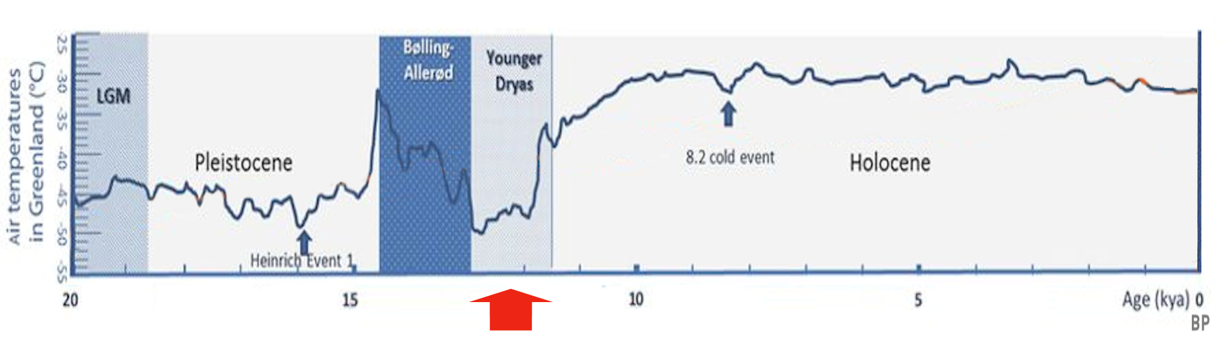
What is the “Younger Dryas,” you might ask? The event itself was a brief return to icehouse conditions at the very end of the Pleistocene Epoch. This kind of funny-sounding name actually references a particular indicator plant, Dryas octopetala, an alpine-tundra wildflower that became more prevalent during this time. We know this because its pollen became more common in lake sediments.

It is called “Younger” because it is the last of three similar sudden cooling phases during  a much longer, gradual, warming from the last glacial maximum. The others are called the “Oldest Dryas” and “Older Dryas.” The Younger Dryas begins after a period of gradual warming that had lasted from 24,000 years ago to 12,900 years ago. For about 12,000 years, the Earth had been slowly warming, emerging from a long icehouse period as had been the cycle since the start of the Pleistocene 2.58 million years ago. Then, quite suddenly, actually in the course of just a few decades (a human lifetime or less), the global climate reverted to an icehouse period for another 1,000 years, until 11,700 years ago.

What caused this particular climatic event is complicated and not fully understood. It is particularly interesting because of the rapidity of the cooling, which has its counterpart in today’s similarly rapid warming at the hand of humans. Humans, however, did not cause the rapid cooling of the Younger Dryas. But, what did? There are three hypotheses worth exploring. None of them are conclusive, but because the question is open, science is at work.

Hypothesis 1: One hypothesis for the onset of the Younger Dryas is the Vela Supernova explosion that took place at that time. In the constellation Vela, a massive star exploded. Energy from this event is suggested as the cause of the observed evidence for the destruction of the ozone layer, changes in nitrogen levels at Earth’s surface and in the atmosphere, megafauna extinctions, and changes in some stable isotopes. However, there is little understanding of how such events could cause these things. So, while you can read about this hypothesis, there is little support for it.

Hypothesis 2: A second hypothesis suggests that a volcano in southern Germany, Laacher See, erupted. An unusual volcano, a “maar lake,” it is today a low-relief crater about 2km in diameter. It is calculated that the eruption at the time would have been large enough to send enough material into the atmosphere to account for the degree of cooling during this period. However, it has not been studied thoroughly enough.

Hypothesis 3: A third hypothesis proposes a bolide impact large enough to cause the climate change observed. A wide variety of evidence exists from sites around the world for their having been such an impact at that time. These include grains of melt-glass and nanodiamonds. What was missing was a crater of the right age. In 2018, under a glacier called “Hiawatha” in northern Greenland, researchers found a massive crater that may fit the bill. At 31km wide, it is not as large as Chicxulub (the dinosaur extinction crater), but represents the effects of what was likely an iron asteroid 1.5km across slamming into the Earth at the time. Its timing is still up for debate, as it could be as old as 100,000 years or as young as 12,900. More research will bring answers.

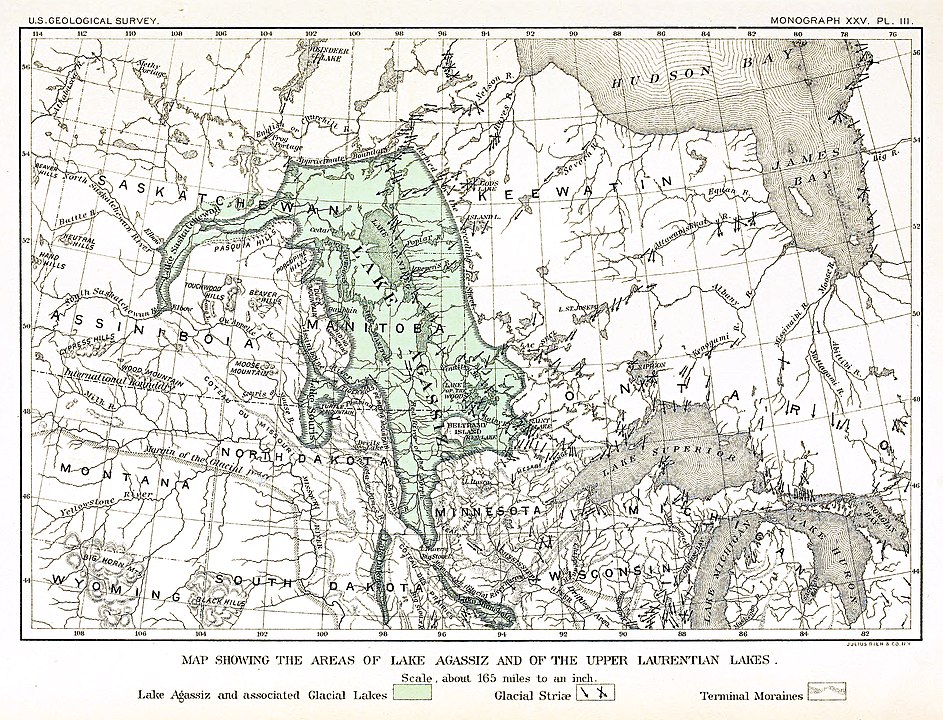
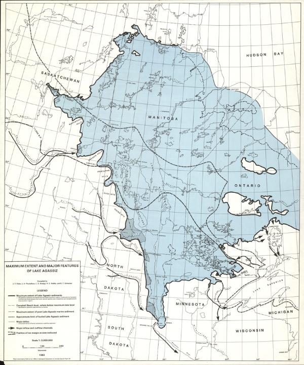
Hypothesis 4: A fourth hypothesis for this abrupt onset of climate change is the emptying of glacial Lake Agassiz in southern Canada into the North Atlantic via the St. Lawrence seaway. Remnants of this post-glacial lake still exist today and include Lake of the Woods, Lake Winnipeg, and Lake Manitoba, among others. Periodically, this lake would be dammed up by ice, allowing fresh meltwater to accumulate over a very large region. There are five identified phases in all in the record. When the glacial dam would burst, massive volumes of freshwater would enter the North Atlantic and disrupt the current thermohaline circulation and significantly alter global climate.

 

The Holocene Epoch

Holocene, from the Greek, means “Entirely New.” For 11,700 years (since 11.7 ka), the climate on our planet has been remarkably stable. Because of this stability, our own species has been able to not only flourish, but to spread well beyond the geographic ranges and biomes to which it was limited during the Pleistocene. While our hunter-gatherer ancestors within the genus Homo have been wielding fire as far back as 1.2 million years, they relied only on what the land provided them for all of that time when it came to food and shelter. That meant hunting game, gathering fruits and plants, and more. The long stability of Holocene climate, combined with our species’ cultural development up to that point, made technologies leading to agriculture, via the Neolithic Revolution, possible. This revolution would provide new sources of food, through the artificial selection of grains and subsequent plants (and animals, eventually), that no longer required consistent or even just seasonal movement. It was possible to settle in one place, develop towns, eventually cities, and the specialization and division of labor. It may have also made it already possible for our species to alter the planet’s climate. More on that in a moment…

Unusual Stability – Sort Of…

Is the Holocene’s climate unusually stable? When compared to other spans of time between ice ages, including the last interglacial (the Eemian), there are many similarities in terms of temperature and duration. The Holocene Epoch is one of the longest interstadial periods on record. This being said, there are some noteworthy departures from this stability that are worth exploring. As of 2018, two of these have been used to further divide our epoch into ages.

Subdividing the Holocene: Climatic Ages

While there have been one or two attempts in past decades to further subdivide the Holocene Epoch, nothing stuck. The Quaternary, in general, is overwhelmingly defined by ice ages. Because Quaternary stratigraphy is overwhelmingly defined by deep sea marine sediments and ice core markers, it is reasonable then to assume the task of subdividing the Holocene Epoch would be no different.

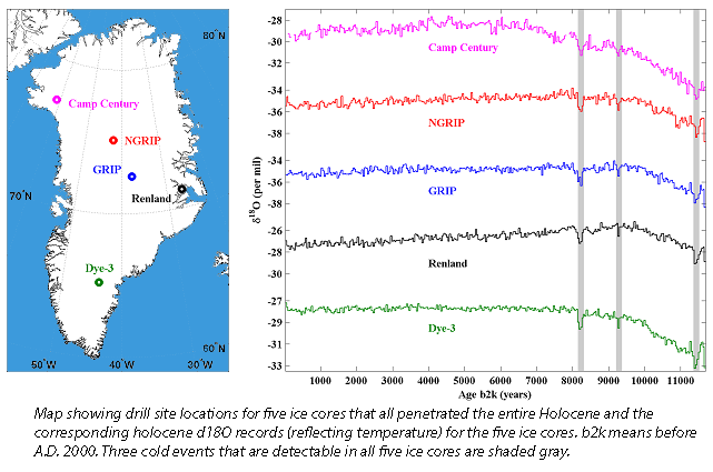
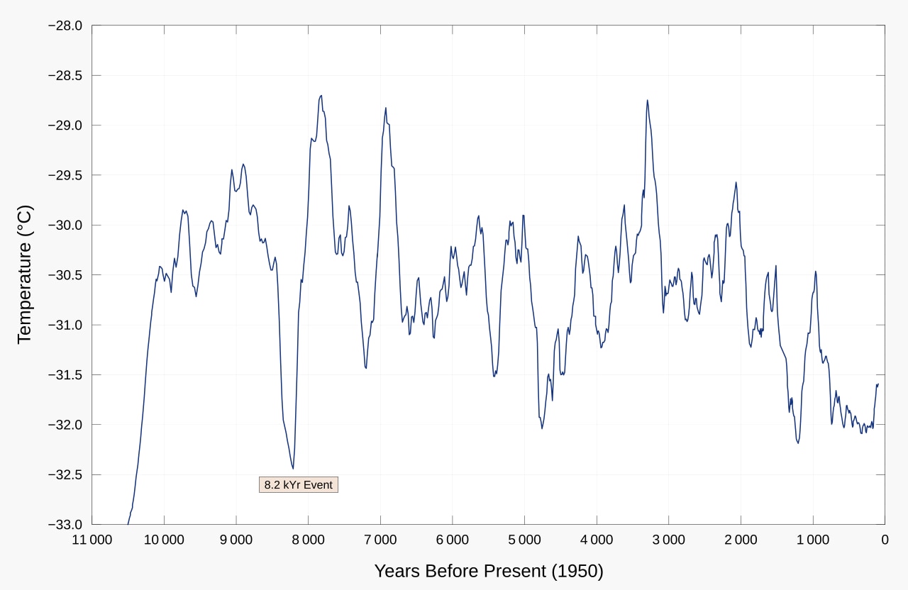
However, the Holocene is not punctuated by long-lasting changes in climate. A three-part division was proposed based upon ice core and cave speleothem data. The base of the Holocene Epoch, the Greenlandian Age, and the subsequent Northgrippian Age, have GSSPs marked in ice cores, NGRIP2 and NGRIP 1, respectively. Our current age, the Meghalayan Age, is recorded in a speleothem record from a cave in Meghalaya, India. Within the boundaries of the Holocene Epoch, two major climatic events of note can be picked out during the 11,700 year long Holocene, one at 8.2ka (ka = thousands of years ago, or kiloannum. “ka” and “ky” are historically interchangeable) and the other at 4.2ka.

The 8.2 ka event – The Greenlandian Age ends and the Northgrippian Age begins

The base of the Holocene begins at 11.7ka with the Greenlandian Stage GSSP recorded in the NGRIP2 ice core. But what happened? Why is it noteworthy? It is located at a depth of 1492.45m where a shift to heavier δ¹⁸O values is recorded. In stable isotope science, we can use the environmental fractionation, or separation, of isotopes of some elements to tell us something about temperature, moisture, or other variables. Because ¹⁶O and ¹⁸O move around in the environment in different and predictable ways, we can use this particularly isotopic pair as a paleothermometer. to understand the Greenlandian/Northgrippian transition, oxygen isotope thermometry is a key. Below is an excellent discussion of the basic science of these methods.

In the ice, according to Walker, et al. (2018),  the change is quite rapid, taking place in just a few years. Accompanying the changes in δ¹⁸O were similarly abrupt declines in deuterium values, a reduction in dust concentrations, and a reduction in Na (sea salt) values. This evidence denotes a sudden cooling, very likely on a global scale, as recorded in central Greenland ice core reconstructions.

At 8.2ky, the Greenlandian Age ends, giving way to the Northgrippian Age. This GSSP is defined by a boundary in the NGRIP1 Greenland ice core at a depth of 1228.67m. Walker, et al. (2018) describe this interval as representing a clear signal of climate cooling during an otherwise warming interval of the Holocene. Recorded in a wide range of proxy records around the globe, it is significant because it is relatively short-lived.

The cause of this event is not entirely certain, though it is typically attributed to the release of fresh, cold glacial meltwater from Lake Agassiz and Ojibway into the north Atlantic. These proglacial lakes were quite large, located between today’s Lake Superior and the Hudson Bay in southern Canada. They are survived today by a wide variety of landscapes, including Lake Winnipeg, Lake Manitoba, Lake of the Woods, and other bodies of freshwater from northern Minnesota well into the Canadian provinces of Saskatchewan, Manitoba, and Ontario.

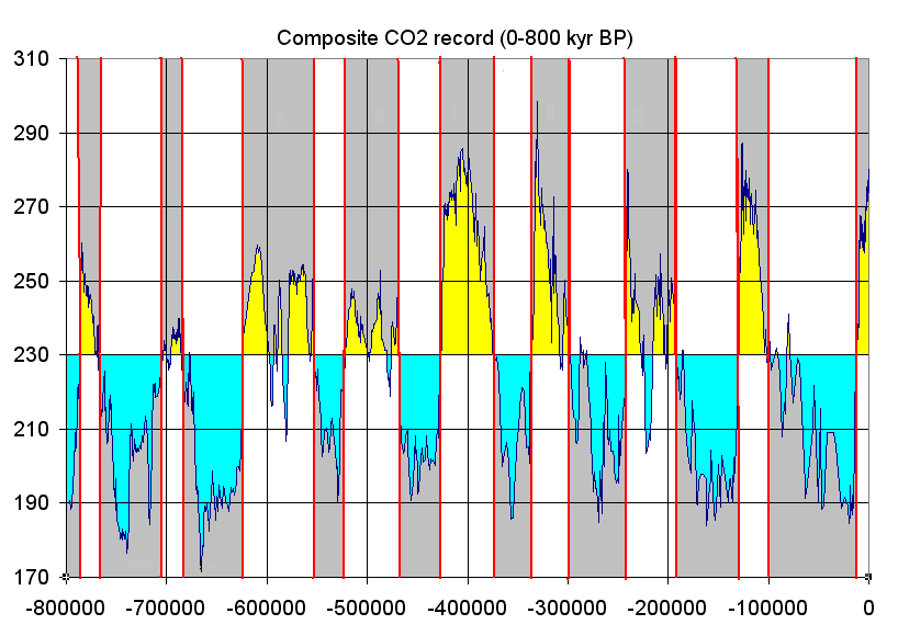
Water likely spilled through the Great Lakes and St. Lawrence Seaway in a great rush, released by a glacial dam. This type of event is called an outburst flood. The sudden infusion of so much cold freshwater into the north Atlantic would have upset the thermohaline circulation in the ocean. This circulation moderates northern temperatures and the shutting off of the current would have caused a significant cooling event, particularly in the northern hemisphere, but with global importance. This cooling could have been as rapid as 3.3°C in just 20 years. Spotty records in tropical regions such as Indonesia also bear records that show a similar cooling, indicating that it was not just an Arctic event. Globally, atmospheric carbon dioxide dropped by 25 ppm over the next 300 years.

The 4.2 ka Event

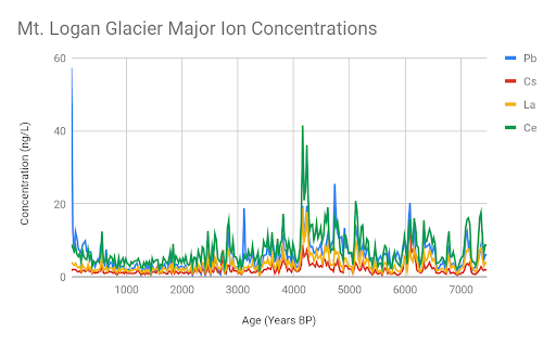
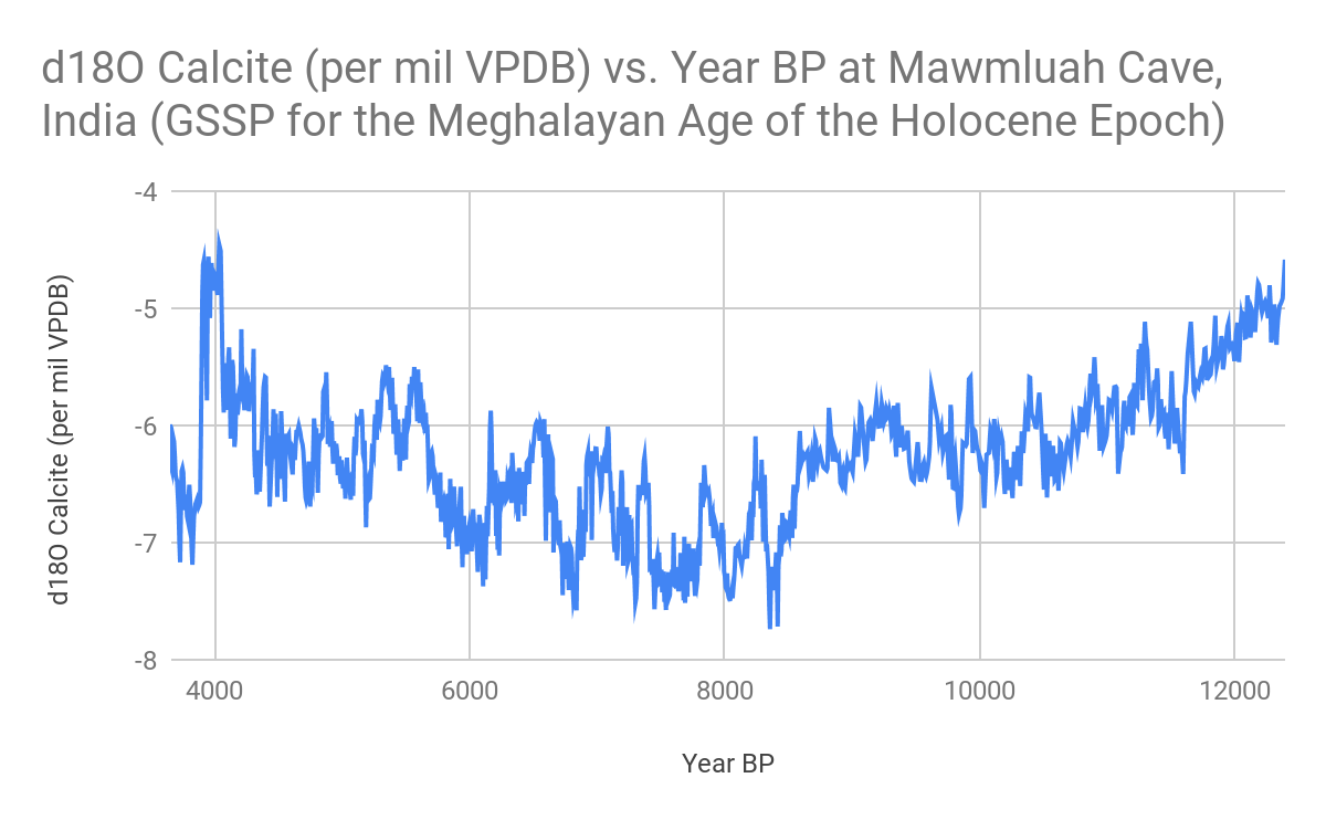
The Northgrippian Age would come to an abrupt end with a another global cooling event, this time accompanied by significant aridification. In 2018, the International Commission on Stratigraphy officially identified the GSSP for the event in a speleothem formation from Mawmluah Cave in Meghalaya, India. As a result, the new age is called the Meghalayan Age. It is the current geologic age in which we live. There is also an auxiliary GSSP contained in an ice core from Mt. Logan, Canada.

At the outset of the Meghalayan, many places around the world became much, much drier. This includes large regions of every continent. Changes in east Indian and Chinese monsoons were triggered, moving patterns further to the south than they had before. With changes in weather patterns that would last well over a century, human civilizations at the time were impacted. The degree of this effect is debated among archaeologists and climatologists, but the 4.2ky event coincides with the end of the Old Kingdom in Egypt, the Akkadian Empire in Mesopotamia, the Lianzhu Culture in China, and the Indus River Civilization in India.

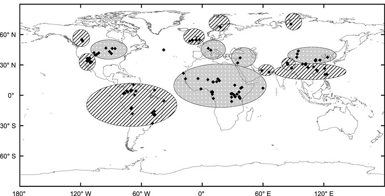
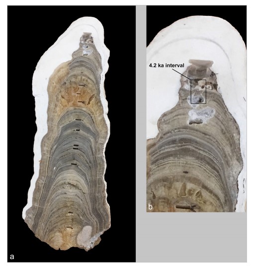
The GSSP itself is marked in the speleothem by a marked reduction in rainfall at 4200 years BP. Evidence from other regions suggests major oceanic and atmospheric changes, particularly in circulation patterns, sometimes referred to as the “Holocene Turnover.” The event appears to have been global. Evidence for this period of aridity is recorded in many locations around the world, including north Africa, the Middle East, and around midcontinental North America. Glaciers record the event in locations like Kilimanjaro, the Andes, and flowstone in Italy. In the northern hemisphere, glaciers re-advanced due to cooling. In mid- to low latitudes, it was marked by aridification in many areas along with disruption of the westerlies, the Indian Summer Monsoon, and the East Asian Summer Monsoon. The resulting megadrought seems to have lasted about 250 years.

This ends the major official divisions of the Holocene. However, the 8.2ky and 4.2ky events are not the only climate “blips” during the epoch. Two other minor ones occur much later on. Ironically, these have received the most attention over the past few decades, so it is possible you have heard of them.

The Medieval Warm Period

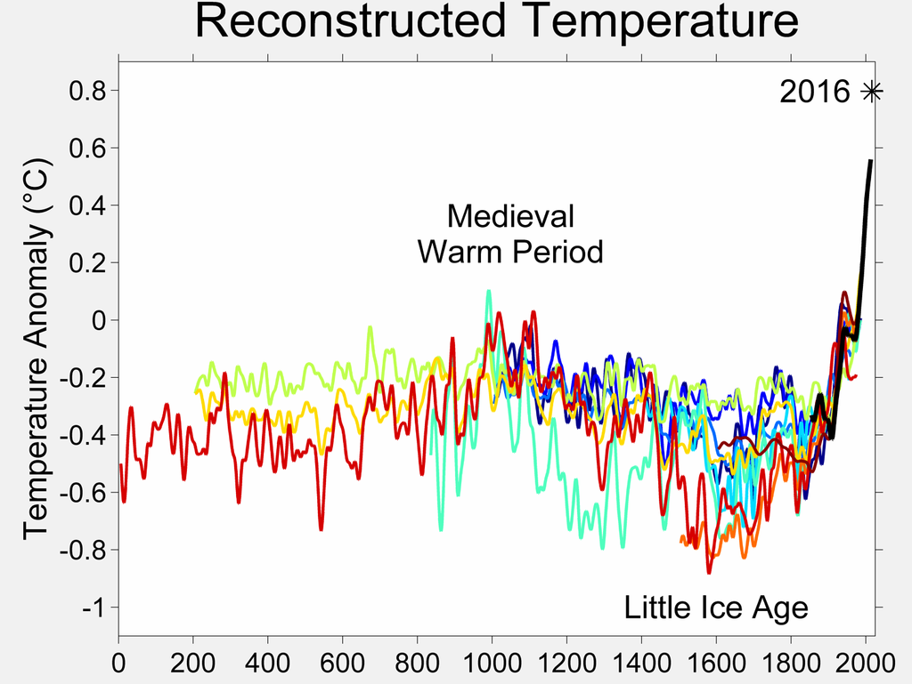
The Medieval Warm Period lasted between the years 900 and 1300 CE. It is also sometimes referred to as the Medieval Climate Optimum or Anomaly. For the north Atlantic region, the climate was marginally warmer than the period following up to the mid-20th century. It can be seen in the GISP-2 ice core from Greenland. Possible causes of this anomaly include changes increased solar activity, decreased volcanic activity, or even changes in ocean circulation. There is not strong evidence that it was a global event.

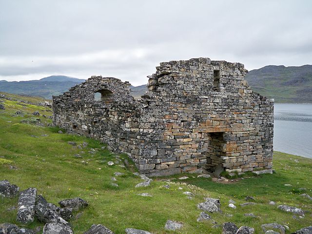
In western culture, the focus on this period is largely due not only to the cultural effects it had on mainland Europe, but as a cause for trans-Atlantic exploration, particularly by the Norse. During this time, groups of Norse colonized Iceland, then Greenland, and eventually reached North America (Newfoundland’s L’anse Aux Meadows) around 1000AD under Leif Erickson. Beginning around 985 CE, Greenland became an important settlement, getting large and stable enough for the Catholic Church to send a Bishop. Walrus tusk, collected for its ivory, was a major export.

Even during this time, however, the Greenland climate was quite harsh, requiring that cattle be contained within stone and earthen barns with walls 10 feet thick for nearly eight months of the year.

The Little Ice Age

Eventually, it became much harder to make a living in Greenland. This was not just due to economics, but also to the onset of the Little Ice Age. As shown in the temperature reconstructions above, this period of cooling occurred directly after the Medieval Warm Period. Again, it was not necessarily global and may have been a regional event in the north Atlantic. It lasted from about 1300 to 1850 CE, the traditional start of the industrial revolution in Britain.

Possible causes have been proposed include the usual suspects: changes in solar radiation, increased volcanic activity, and changes in ocean circulation, among others. Even decreases in human population has been proposed as a cause, due to the Black Death plague that killed millions of Europeans during the 14^th century. In any case, life in Europe during this time was a mix of hardship, cultural Renaissance, and exploration. The latter was largely motivated as a  search for resources to supply a now very resource-poor continent. The cultural and climatic ramifications of this exploration echo into the present day.

The Anthropocene

Officially, this should be the end of the story. Up to this point, we have explored how the the Quaternary Period, its epochs and ages, have been subdivided using GSSP markers from the past that are clear and can be agreed upon by specialists (more or less). The distinction between GSSPs housed in ice marking boundaries in the Quaternary versus more traditional stratigraphic markers in rock that mark the rest of the time scale does not require a great leap of understanding. But is this the end of the story of our modern geologic time?

Humans are a force of nature. As a single species and in a very short period of geologic time, we have altered the climate, fragmented the rest of the biosphere, and are likely the cause of a sixth mass extinction. Here is a short list of anthropogenic (human-caused) effects on our global environment that, since at least the mid-20th century, are amplified with enough intensity that some have been led to argue that we are in a new geologic moment:

• • Humans have been and are altering the composition of our atmosphere. This has been going on since at least 1750 with the onset of the Industrial Revolution in Great Britain, but perhaps as far back as the Neolithic Revolution around 10ka. This includes greenhouse gas emissions such as carbon dioxide (CO₂) and methane (CH₄), but also chemical and particulate emissions from other industrial, commercial, and household sources. These include black carbon, chlorofluorocarbons (CFCs), HCFCs, etc.;
  • Humans are changing the chemical physical composition of the hydrosphere. Again, this has been occurring in increasing intensity since 1750. It includes direct pollution of marine settings chemically and through sewage and litter, as well as indirectly through seawater absorption of excess CO₂ from the atmosphere (ocean acidification). Surface freshwater and groundwater resources have also been impacted, sometimes catastrophically;
  • Humans are changing the layout and composition of the terrestrial and marine biosphere. This alteration includes overhunting of select large game over time, fragmentation of forest and habitat more generally, alteration of landscapes from wild to cultivated for agricultural purposes, and selective elimination of “pests.” It also includes the rapid spread of non-native species to areas due to human commerce. This has led many to hypothesize that we have entered a sixth period of mass extinction, akin to the “big five” (discussed in other chapters);
  • Humans are altering the surficial makeup of the geosphere. We are altering coastlines, slopes, and other geomorphology. Our agricultural practices contribute to soil loss, desertification, and the drying up of surface water bodies;
  • Humans are altering the exosphere through the addition of space debris;
  • Secondary, often amplifying feedback effects, result from all of these. That is, a direct alteration of one environmental variable often leads to a indirect change in another that is not being directly affected by humans. Many times, such effects amplify the negative impacts of the initial human activity through system feedbacks. An example is the human addition of CO₂ to the atmosphere that leads to warming, which leads to the melting of ice, which leads to lower polar albedo, which leads to more absorption of solar radiation, which leads again to greater warming.

In the history of our planet, it is possible that no single type of organism has ever had this magnitude of an impact (One possible contender is the oxygenation of the atmosphere by cyanobacteria during the Proterozoic). It is definitely the case that the impact of a single species has ever led to change occurring at the rates the planet is now experiencing. For a small taste of this, check out the “Wrecked Wrack” image below. This represents the trash picked up along a 0.8 km (0.5 mile) stretch of the beach on South Padre Island, Texas. These materials could be described variously as anthropogenically-unique materials. You might one day call them technofossils, as they are some of the objects likely to end up as a part of our modern “fossil” record.

These realities are alarming, but also scientifically verifiable. The material pollution documented above is being deposited in sedimentary basins today. It will likely enter the geologic record as a distinct indicator of humanity’s time on the planet.

Because of this, in 2000, atmospheric chemist Paul Crutzen and limnologist Eugene F. Stoermer proposed the creation of a new period of time, the Anthropocene, to mark the age of humans and their effect on the planet. This idea was not entirely new. Soviet scientist Vladimir Vernadsky, in 1938, wrote of human scientific thought itself as a geologic force, using the term Anthropocene for our modern time. The term had also been used by later Soviet scientists as a way to refer to the Quaternary as a whole. Stoermer had been using the term himself since the 1980s, as a way to refer to human impacts on the Earth. The modern use of the term as we will read about it below goes back to a story Paul Crutzen tells of being at a conference where at one point someone mentioned something about the Holocene. Feeling that using this term to describe our current time was wrong, he suddenly stated, “No, we are in the Anthropocene.” By 2008, geologist Jan Zalasiewicz wrote in GSA Today that defining an Anthropocene Epoch is now appropriate. Since then, the ICS has created an “Anthropocene Working Group” which, in 2016, voted to proceed toward identifying a GSSP to define the beginning of an Anthropocene Epoch.

This would mean an end to the Holocene Epoch and Meghalayan Age sometime in our recent past, perhaps within the last 100 years. Indeed, while various start dates have been proposed, some of which will be discussed below, the greatest consensus is forming around a start date of 1950, a date marking a peak in radionuclide fallout from global nuclear testing as well as the start of a time period referred to as “The Great Acceleration.” Since 1950, this acceleration is seen in data wide-ranging enough from the Earth system to cultural and economic trends. Overall, human impacts have led to exponential increases in these trends due to the force of human population growth and increasing development through the use of fossil fuels.

Challenges and Implications

After reading this case study, you may already have identified what may be the greatest philosophical hurdle in defining a new epoch based upon human activity. That is: if our model of geologic time is based upon defining GSSPs using traditional stratigraphic markers (including in ice), how can we define an entirely new geologic age of any kind using markers that may not yet be a part of the geological record? This may seem to go against our model of geologic time and the rules we have used to create it. Does this new designation follow the model and its rules closely enough to be accepted as valid by the scientific community?

A second issue is one of vanity. While certainly the vast majority of the scientific community understands the magnitude of the human impact on the environment, is the definition of a new epoch truly useful in the traditional geologic sense? Or, is it more an exercise in defining our age as a way of encouraging political or social movement toward solving major environmental challenges? How will geologists make use of this epoch – an epoch that may have so far only lasted about 70 years – a blip barely registering in the whole of geologic time? Even if the standard of comparison is the whole Quaternary Period, 70 years is not much.

These are tough academic — even epistemological — questions. The issue is being debated right now among geoscientists. Here, we can only ask the questions rhetorically, but they will beg an answer at some point in the future.

Finding a Start Time

In a practical sense, the Anthropocene Epoch would need to be defined by a GSSP just like any other boundary on the geologic time scale. This means, succinctly, a geologically-distinct stratigraphic marker that is temporally distinct, clear in the geologic record, easily studied, accessible, and eventually can be ratified by the ICS through agreed upon rules and policies. This has led to lively debate within the ICS’s Subcommission on Quaternary Geology, its Anthropocene Working Group, and among other scholars whose fields of work directly inform the debate. Due to the unique nature of the proposed Anthropocene Epoch and the focus on human impacts, debates over this change have extended beyond just geoscientists. Archaeologists, anthropologists, and specialists in other fields have tossed their ideas and contentions into the fracas. While this has certainly made the identification of a GSSP for an Anthropocene Epoch a whole lot more exciting than the usual act of defining a GSSP, it has also muddied the waters.

The big question is, when do you mark the start of anthropogenic effects? When so much of the Holocene is marked by the story of our species, how do you choose where to draw the line?

The Industrial Revolution: 1750

Because of the clear effects of fossil fuel combustion and their clear, well-documented effect on our changing climate, the start of their widespread usage by humans presents an obvious “go to” time candidate. Data, particularly regarding greenhouse gas CO₂ emissions since then would seem to support this start date as a clear favorite.

Instrumental carbon dioxide records from locations like NOAA’s observatory atop Mauna Loa, Hawaii, have only been collected for a few decades. The graph above is reconstructed from other proxy data, as is the data for human emissions. Still, this would seem to be pretty convincing, particularly if we extend carbon dioxide emissions a bit further back in time.

When examining the chart above, the case for 1750 as a start date for an Anthropocene Epoch seems quite clear.

However, there are a few problems. One of these is that the main data of record is atmospheric carbon dioxide, and that alone. While this is not in itself unusual, identifying a GSSP using the usual rules is challenging. For one thing, it is not necessarily recorded in ice at this point, or reliably, particularly due to the practical issue of global warming having melted so much of the recently deposited ice, and likely to melt a lot more of it in the future. But if the GSSP cannot be identified in ice, it needs to be found in some other solid Earth record that is well-preserved and accessible. While it is possible that an anthropogenic peak in black carbon (such as soot from power plants and factories) could be potentially identified, the sediments that contain it are not yet rock.

There are other problems, but just these few illustrate the challenge of arguing for 1750 as a start date. The start date makes sense culturally and in some limited data, but a GSSP is really hard to identify.

Besides – why start at 1750 when it can be argued that humans have been altering the atmosphere for much, much longer?

The Ruddiman Hypothesis: The Neolithic Revolution at ~10,000 BP

In 2005, William Ruddiman, then a Professor of Environmental Sciences at the University of Virginia, published a book (Plows, Plagues, and Petroleum: How Humans Took Control of the Climate) that argued for a much earlier start date to the Anthropocene. Ruddiman’s idea is known as the “Early Anthropocene” hypothesis, since he argued that human-induced changes in atmospheric greenhouse gases actually began with the advent of agriculture, the Neolithic Revolution.

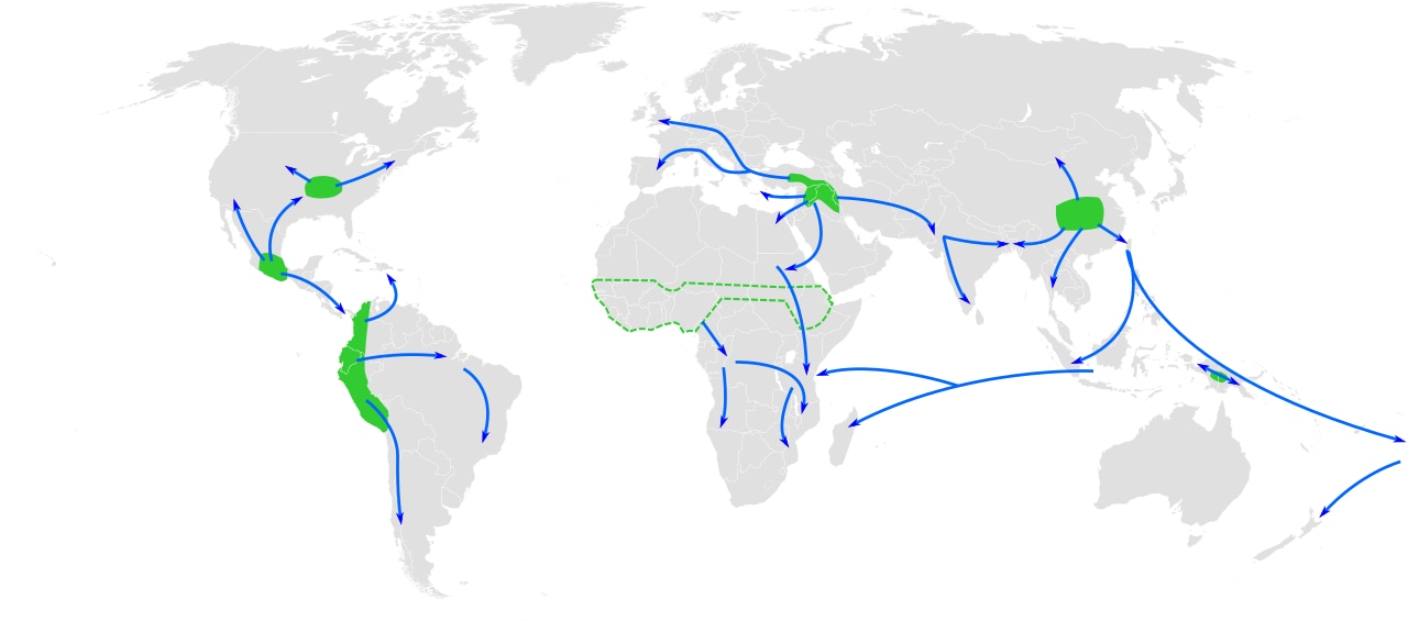
The idea is very similar to the case for 1750. Human technological innovation has led to major changes in the Earth system. It is just that these effects were from a switch from hunter-gatherer nomadic lifestyles to more sedentary agricultural lifestyles. Agricultural innovations associated with the Neolithic Revolution, such as the domestication of cereal crops beginning around 10,000 BP in the Near East “Fertile Crescent” region containing the Tigris and Euphrates Rivers (modern Iraq, parts of Iran and Turkey, Syria, and Israel/Palestine) and parts of the Mediterranean Sea coast. This particular innovation would develop independently in several other locations, including central China, Egypt, Mesoamerica, central North America along the Mississippi River, and coastal South America. While cereal grain domestication occurred earliest in the Near East, independent development of agriculture in other areas allowed the sharing of technological innovations around the globe.

Prehistoric agriculture, as is still done today, involves the widespread clearing of land and burning of debris. The clearing of land removes vegetation, a natural carbon sink, and its burning then releases carbon back into the system, pumping carbon dioxide into the atmosphere. Some of this carbon had been stored for thousands of years. Such burning for agriculture can still be seen today in places like Indonesia, where massive areas of land are being “slashed and burned” for the planting of palm oil plantations, very often illegally. This burning of debris and accumulated peat is a major source of anthropogenic greenhouse gas emissions today also.

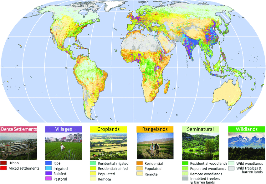
However, widespread burning of debris is not only associated with agriculture. Humans have been using this technique for much longer to burn away underbrush in forests to aid in hunting. When early Europeans arrived in the Americas, for instance, it was observed that it was possible to drive a wagon with four horses side by side with little trouble. Indigenous Americans were able to efficiently clear large swaths of forest in this way. When European disease and warfare drove them out of their lands or killed them altogether, Europeans simply cut down forests or, in the case of forests left standing, did not have a cultural practice of burning underbrush. Thus, it accumulated. Human alteration of the environment over time has turned biomes into anthromes.

Around 8,000 years ago, humans domestication of animals began in earnest. Ruminant animals, in particular, the contributed large amounts of methane to the atmosphere. These animals are still a major source of anthropogenic methane today. Within the rumen of these animals, a group of Archaea known as “methanogens” (Euryarcheota), produce methane from the chewed-up vegetation the animals have eaten. The process is known as enteric fermentation. Contrary to popular imagination, these animals pass this gas into the atmosphere through belching, rather than flatulence. Cumulatively, the amount of methane is very significant.

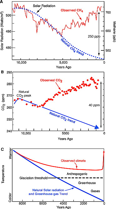
Both of these gases are potent greenhouse gases. The “Early Anthropocene” argument uses climate modeling to make the case that the collective developments associated with human agriculture were enough to forestall entering a glacial period. Further, this would mean that the climate changes we are experiencing today are simply a more rapid manifestation of climate changes resulting from technological innovations our ancestors made thousands of years ago.

How would this work as a GSSP? This would place the start date for the Anthropocene Epoch at 10,000 BP. With the Holocene Epoch GSSP identified at 11,700 BP, this would either reduce the length of the Holocene to a mere 1,700 years, or make a good argument for either renaming it or just re-imagining how we view the Holocene altogether, thus tossing out the Anthropocene Epoch concept entirely. As for a physical stratigraphic boundary in the rock record, archaeological data could be used to mark a cultural progression, but this would be a significant departure from convention. In reality, we are left with the same problem with using 1750 as a start date. It is nearly impossible to identify a physical location where a rock formation accuratey records this transition.

Is there a time when humans really made their mark in a more explosive manner?

The Atomic Age: 1950 and the “Great Acceleration”

21 days before the first atomic bomb was dropped on the Japanese city of Hiroshima, the first test of an atomic bomb took place near Alamogordo, New Mexico. On July 16^th, 1945, the Trinity Test resulted in a 22 kiloton explosion. Below is some of the only footage of that test that exists. The explosion itself can be seen near the end of the clip.

The explosion itself had a yield equivalent to 15,000 to 20,000 tons of TNT. In the years following World War II and until 1963, eight countries developed and tested nuclear weapons. Post-1963, further tests were conducted by Pakistan, India, and North Korea, but these are much more limited in scope. Still, the radionuclide fallout from these early tests, beginning with Trinity, are verifiably recorded in the geologic record.

These nuclear tests represent a technological innovation with power beyond anything else humans have harnessed. Because of this, and because of the global distribution of the radioactive fallout, the emerging consensus is that this period of nuclear testing, beginning in 1945 and extending into the early 1950s, is the ideal temporal horizon to use for the start of the Anthropocene Epoch.

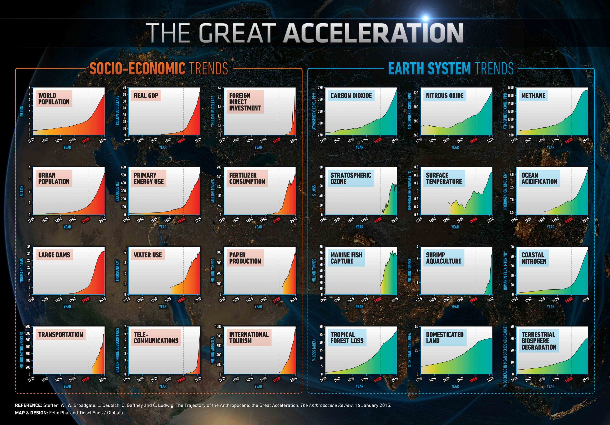
Radionuclide accumulation in the geologic record is not the only significant anthropogenic signal to accumulate from this point. In 2015, scientists with the International Geosphere-Biosphere Programme released their latest data set for what they deem “The Great Acceleration” (Steffen et al., 2004). The idea here is that the rapid and massive growth of socio-cultural trends and Earth system trends beginning around 1950. The advent of the nuclear age and a new source of energy, helped usher in a global industrial revolution that continues its rapid expansion to the present. Socio-economic trends such as human population growth, GDP, fertilizer consumption, urbanization, etc. have put major pressure on the environment. Resulting environmental trends include increases in atmospheric carbon dioxide, nitrous oxides, methane, stratospheric ozone, lower ocean pH (acidification), and forest loss. When graphed, data for all of these groups of variables produce exponential curves, largely beginning around 1950. While not all of these trends will make ideal geologic records, they certainly argue that a rapid increase in anthropogenic population, activity, and energy production has made a lasting impact on the planet.

The case for an Anthropocene Epoch start date around the year 1950 is compelling. There is a clearly different trend of change in the global natural environment with human activities as the sole or primary driver.

As of this writing, the hunt is still on for a GSSP. It is not unusual to identify a moment in time before a GSSP marker is found, as there are still boundaries on the geologic time scale that completely lack a GSSP to physically define them. Nevertheless, there are a handful of locations being actively pursued as having the potential to contain the key marker for an Anthropocene Epoch. One candidate is Crawford Lake, Ontario, Canada, where its depth precludes complete mixing of layers, allowing its bottom sediments to lie undisturbed. Other sites include an Antarctic ice core, cave deposits in Italy, coral reefs in the Caribbean and Australia, and a peat bog in Switzerland. If present, the signal at all of these locations is a mix of chemical markers consistent with radionuclide fallout, such as carbon-14 and plutonium-239, but also including other potential markers like organic pollutants, microplastics, and fly ash.

Ratifying a GSSP

The currently agreed-upon temporal marker for the end of the Holocene Epoch and the start of the Anthropocene Epoch is the year 1950. As data documenting the so-called “Great Acceleration” discussed above shows, anthropogenic effects on the environment have increased by orders of magnitude over background rates, been very sudden, progressed very rapidly, and have altered the natural environment enough to be recorded in the geologic record, beginning with radionuclide fallout. The Anthropocene Working Group documents >+1 order of magnitude increases in sediment transport due to urbanization and agriculture; marked and abrupt perturbations in biogeochemical cycling of carbon, nitrogen, phosphorus, and various metals; global warming; global (eustatic) sea-level rise; ocean acidification and proliferation of “dead zones;” rapid biosphere change on land and sea; habitat loss, hyper-predation/hunting, increase of domestic animal populations, and widespread expansion of invasive species; and the abundance and spread of new human-designed substances such as fly ash, plastics, concrete, and technofossils (Anthropogenic Working Group, 2020).

Because these alterations of the Earth system will persist for many millennia (some will be permanent), the Anthropocene Working Group has established that these materials are sufficient to produce durable geologic strata that are sufficiently unique to be separate from Holocene stratigraphy. Because of all of this, the Anthropocene Working Group voted on May 21, 2019 and answered in favor of the following questions at the International Geological Congress in Cape Town, South Africa:

1. 1. Should the Anthropocene be treated as a formal chronostratigraphic unit defined by a GSSP? 29 members voted in favor, 4 voted against.
   2. Should the primary guide for the base of the Anthropocene be one of the stratigraphic signals around the mid-twentieth century of the Common Era (i.e., circa 1950)? 29 voted in favor, 4 voted against.

These questions now guide the future work of the ICS’s Anthropocene Working Group. Current work is focused on identifying a GSSP for the Anthropocene Epoch. Candidate locations will certainly be proposed, vetted, and voted upon. The progression from merely suggesting the idea in 2000 to voting on going forward with a formal proposal has only taken 18 years. It is very possible that, within the coming decade, you may find yourself in a new geologic epoch.

Concluding Thoughts

Before we began this case study, we defined three important questions about how we define geologic time:

1. 1. How do we use the geologic time scale as a model?
   2. How do we make changes to this model?
   3. How can we use this model to help us define our own time?

You should be able to provide your own answers to these questions. As we have explored some Quaternary quandaries regarding how to apply the model of geologic time, GSSP development, and more, it should be clear that it is not a perfect model. Like all good models we develop to explain what we observe and test in nature, it is flawed at present, but nonetheless quite useful. Keeping this open-minded philosophy about time is important. We can continue to improve the model only if we are aware of its shortcomings or failures. However, the geologic time scale and the techniques we use to create it provide us with powerful resources to help us test important questions about our planet’s past and our own humanity.

Further Reading

Anthropocene Working Group (2020). Working Group on the Anthropocene.

Ellis, Earle (2019). To Conserve Nature in the Anthropocene, Half Earth is not nearly enough. One Earth 1.

Head, Martin J. (2019). Formal subdivision of the Quaternary System/Period: Present and Future Directions. Quaternary International 500:32-51.

Ruddiman, William F. (2003). The Anthropogenic greenhouse era began thousands of years ago. Climate Change 61:261-293.

Ruddiman, William F. (2005). Plows, Plagues, and Petroleum: How Humans Took Control of the Climate. Princeton University Press.

Saavedra-Pellitero, Mariem, Baumann, Karl-Heinz, Ullermann, Johannes, and Frank Lamy (2017). Marine Isotope Stage 11 in the Pacific Sector of the Southern Ocean; a coccolithophore perspective. Quaternary Science Reviews 158.

Steffen W., Sanderson A., Tyson P.D., Jager J., Matson P.A., Moore B. III, Oldfield F., Richardson K., Schellnhuber H.J., Turner B.L. II, and R.J. Wasson (2004). Global Change and the Earth System. IGBP Global Exchange.

Walker M., Head, Martin J., Berkelhammer, Max, Bjorck, Svante, Cheng, Hai, Cwynar, Les, Fisher, David, Gkinis, Vasilios, Long, Antony, Lowe, John, Newnham, Rewi, Rasmussen, Sune Olander, and Harvey Weiss (2018). Formal ratification of the subdivision of the Holocene Epoch (Quaternary System/Period): two new Global Boundary Stratotype Sections and Points (GSSPs) and three new Stages/subseries. IUGS Episodes Journal of International Geoscience 41(4):213-223.

Walker, M., Gibbard, P., Head, M., Berkelhammer, M., Björck, S., Cheng, H., Cwynar, L., et al. (2019). Formal Subdivision of the Holocene Series/Epoch: A Summary. Journal of the Geological Society of India, 93 (2), 135-141. https://doi.org/10.1007/s12594-019-1141-9

Wang, Jianjun, Sun, Liguang, Chen, Liqi, Xu, Libin, Wang, Yuhong, and Xinming Wang (2019). The abrupt climate change near 4,400 yr BP on the cultural transition in Yuchisi, China and its global linkage. Scientific Reports 6:27723.