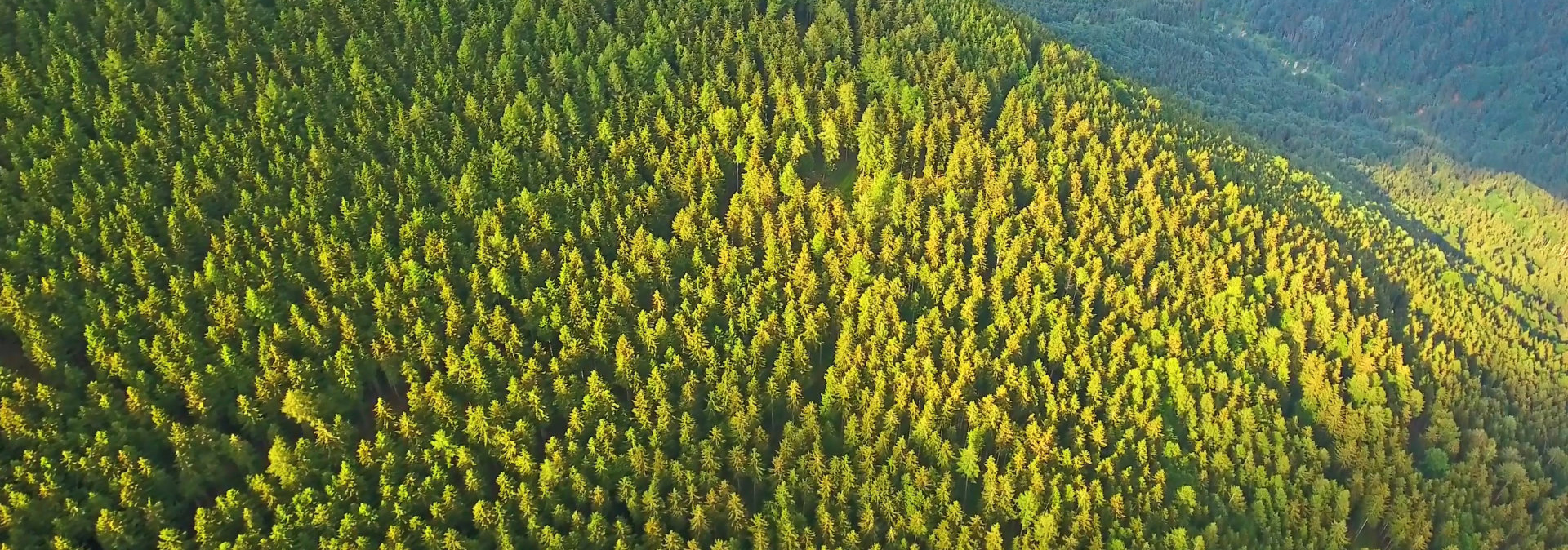
Photo by Roland Sims, CC-BY via Flickr.
Photosynthesis and respiration
Photosynthesis and its sister reaction respiration are key biogeochemical processes in the Earth system. The simplified chemical equation for photosynthesis is:
CO2 +H2O → C6H12O6 + O2
(Requires a lot of energy input, from the Sun)
In other words, the Sun’s energy can cause carbon dioxide to react with water, producing glucose (a sugar) and free oxygen. This reaction is facilitated by living organisms, principally cyanobacteria, algae, and plants {LINK TO PLANT CASE STUDY}. The glucose is the point of the reaction for these organisms, while the oxygen is just an incidental waste product.
For respiration (or its inorganic equivalent, combustion), just flip the equation around and run it in reverse:
C6H12O6 + O2 → CO2 +H2O
(Releases a lot of energy)

Every green plant you have ever seen is actively doing photosynthesis while sunlight shines on its leaves, and the same is true for primordial cyanobacteria and floating phytoplankton in the oceans. Collectively, these organisms are powerful agents of geochemical change: they extract CO2 from the atmosphere, shucking off its oxygen as waste, and use its carbon to build their bodies.
Today, this effect can be measured in real time: photosynthesis in the northern hemisphere summer pulls about 6 ppm of CO2 out of the air. That’s about 1.5% of the total atmospheric pool of CO2! There is not as much land in the southern hemisphere (and much of it is desert), so the CO2 drawdown effect is not as large during the austral summer. It is most pronounced between April and September of each year.
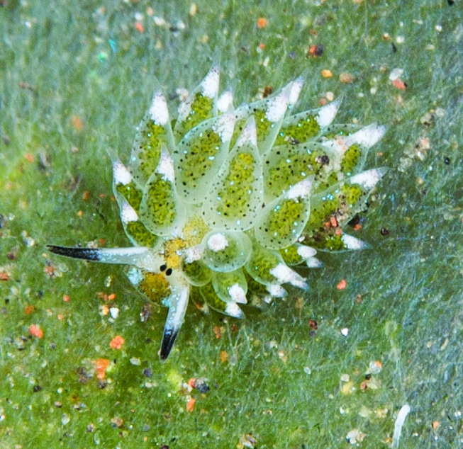
Photo by prilfish, CC-BY, via Flickr.
When animals eat algae or plants, they aren’t doing it to be mean. They are doing it because they will die if they don’t. Unlike autotrophic plants, animals are heterotrophs – a word that means they need to eat. Eating is an act whose intention is to grab some of the plants’ stored energy and use it to drive the animal’s own life: moving, growing, reproducing. As a general rule, animals are not capable of photosynthesis. Eating is their only option. Curiously though, in multiple lineages, some animals have figured out how to host photosynthetic cyanobacteria or algae within their bodies as endosymbionts.
Let’s circle back now to photosynthesis. Driven by the energy in sunbeams, plants suture carbon dioxide to water, making glucose, and ejecting much of the oxygen as waste. But trees are not made of glucose. Instead, they bulk up by converting glucose into cellulose via this reaction:
C6H12O6 + C6H12O6 + C6H12O6 + C6H12O6, etc. → (C6H10O5)n + H2O
Cellulose is a much more durable compound. Non-woody plants such as grasses are capable of projecting upward from the ground because cellulose in their cell walls provides structural support. Along with lignin, cellulose makes up the bulk of trees and other woody plants. It’s wood. Wood makes up the bulk of the planet’s biomass (450 Gt of carbon, about ~82% of the total).
Wood is capable of being oxidized by organisms, but not especially rapidly. Fungi and bacteria can break it down, given enough time. Depending on the species of wood and levels of moisture and ambient oxygen, this decomposition can take a year or several centuries. Herbivores such as termites and cows host symbiotic bacteria in their guts which can break down cellulose more rapidly, but that’s not a trick that humans can pull off! If we decide to oxidize wood quickly, we burn it.
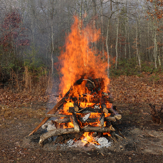
Callan Bentley photo.
We have probably all experienced fire. When you enjoy a bonfire, campfire, or the radiant heat of a woodstove, you’re reversing the photosynthesis reaction via the secondary product of wood. All that warmth, all that orange and yellow light, all those loud crackling noises – these are various forms of energy that are released as the bonds holding together cellulose and lignin are broken. For most wood available to most people, that energy was captured in the past few years or decades.
The same is also true when we burn ancient plant biomass – though not “wood” or “cellulose” any more, ancient plants can provide long-term stores of ancient carbon. Let us next examine how these “fossil fuels” form, and what the implications are of their formative processes, specifically for the atmosphere and biosphere.
Carbon burial
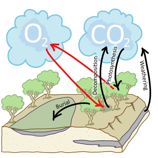
Callan Bentley cartoon.
What must happen next is for plant biomass to be built up through photosynthesis and then buried under sediment before it gets a chance to rot or burn.
Consider this diagram, which highlights some of the fluxes (flows) between the atmosphere, plants, and layers of sedimentary rock. Plants pull CO2 from the atmosphere and release O2 as a waste product. The O2 will eventually react with the plant carbon through decomposition, unless the plant matter is buried. Once buried, it is isolated from free oxygen; it cannot decompose. Its carbon then becomes part of sedimentary rocks, and is locked in the geosphere until uplift (often, mountain-building) brings it back into contact with atmospheric oxygen. This allows it to be weathered (re-oxidized).
What is the impact on the atmosphere of this natural carbon sequestration? It all depends on the timescale over which the carbon remains isolated from the atmosphere, deep in the crust. For our purposes, it makes sense to consider timescales of tens to hundreds of millions of years.
Impacts on the cryosphere and biosphere
Let us consider the impacts of carbon burial on three phenomena: fire, climate, and animal physiology.
Fire
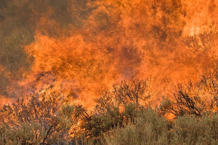
US Fish & Wildlife Service photo.
We listed a few examples of anthropogenic fire above, but fire is also a natural part of the modern Earth system. Wildfires can be sparked by lightning strikes or volcanic eruptions. They are more likely to ignite and to spread in areas that are temporarily warm and dry, but have seen wet enough conditions in the past to build up a supply of plant fuel. Combustion occurs when the plant tissues react with atmospheric oxygen, and release the carbon in the plants back into the atmosphere as CO2.
So oxygen is a pre-requisite for wildfire, and oxygen levels have changed throughout Earth history. How much oxygen is necessary? It turns out that fire requires at least 13% O2 in the surrounding atmosphere. Over the long-term, our planet has bulked up the free oxygen content of its atmosphere, from an initial 0% to the current ~21%. It is estimated that the critical 13% threshold was crossed in the Silurian. Two lines of evidence support this interpretation:
-
- The oldest terrestrial plant fossils are spores that date to the Ordovician, suggesting colonization of the land surface by organisms akin to club mosses. These plants provided fuel to burn, but also shelter for animals. The oldest terrestrial animal fossils date to shortly thereafter. As plants colonized the land, they led to more of the planet’s surface being devoted to (incidental) oxygen production. It is thought that oxygenation of the atmosphere would also have led to the development of an ozone (O3) layer, which would have enabled animals to spread across the land due to lowering the influx of harmful ultraviolet radiation from the Sun.
-
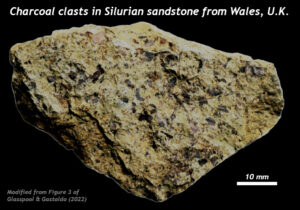
Charcoal clasts in Silurian sandstone from Wales.
Modified from Figure 3 of Glasspool & Gastaldo (2022).By 420 Ma (Silurian), charcoal starts showing up. Charcoal is a carbon-rich version of what used to be wood, but all the water and volatile components have been driven off through heating it in the presence of limited amounts of oxygen. It is our first evidence that fires had started burning on Earth.

With the exception of a “gap” in the mid-Devonian, charcoal has been a common constituent of terrestrial sediments for the rest of the Phanerozoic Eon. Thanks to the rise in oxygen levels, fire has become a standard phenomenon on the surface of Earth. So the burial of plant biomass preserves some carbon for the future, but leaves behind oxygen at the surface, and that oxygen that makes it more likely for unburied plants to burn.
Ice
The greenhouse effect needs a quick recap in order to understand what happens next.
Callan Bentley cartoon.
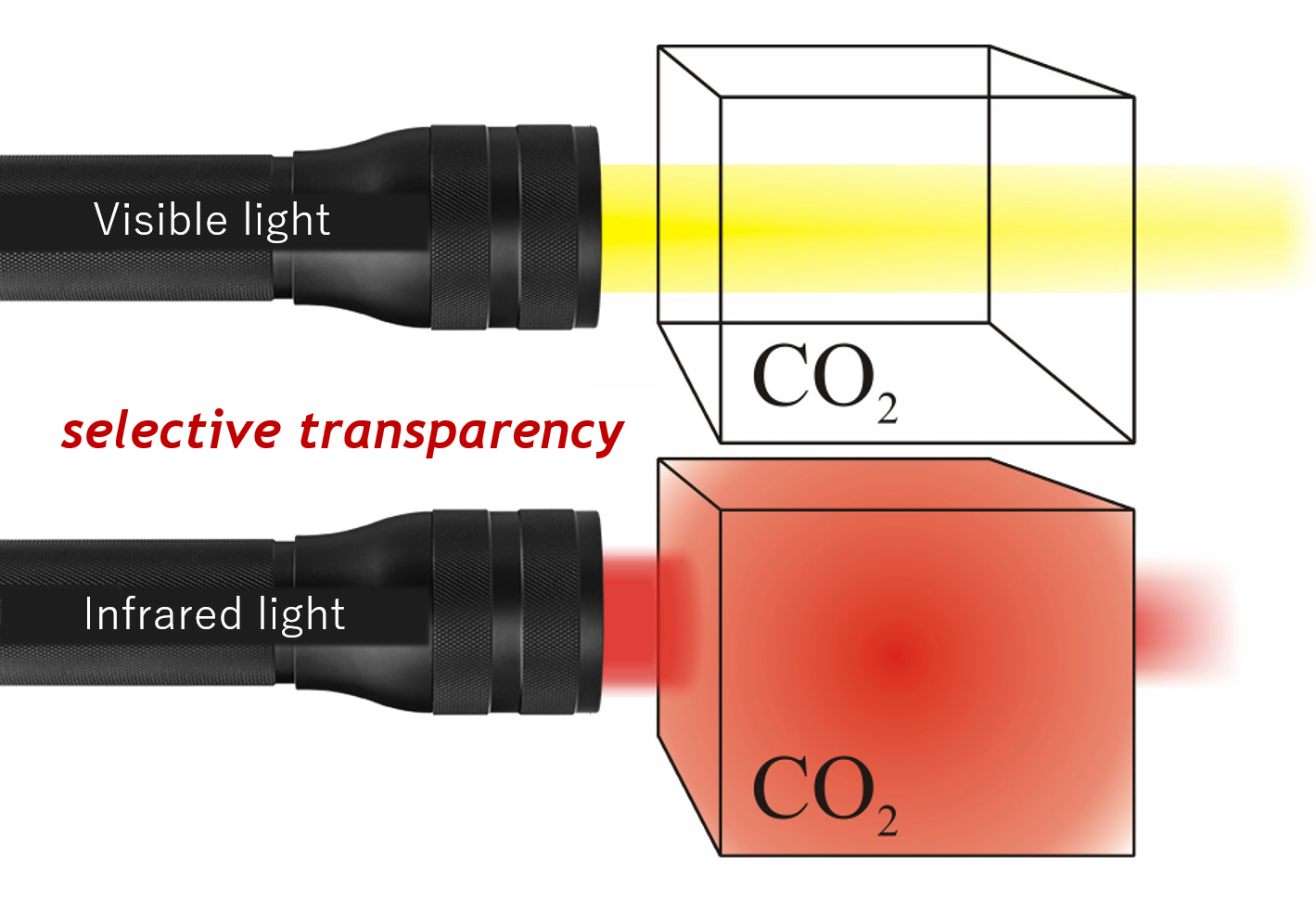
CO2 is an invisible gas. But it’s only invisible to the visible wavelengths of light. Under other wavelengths of light, it shows up as a dense foggy cloud. Specifically, infrared light cannot pierce through CO2 – the infrared light’s energy is absorbed and re-radiated in a random direction. Examine the cartoon illustration of this idea at right: When a beam of visible light is directed through a glass box containing CO2, it all passes through to the other side. But when infrared light is shone through instead, it gets stopped, and so less than 100% makes it across to the far side of the box. So CO2 is selectively transparent to different wavelengths of light.
This matters intensely for the regulation of Earth’s climate. Though the planet is irradiated by visible wavelengths of light, Earth materials absorb that light, and warm up. They then re-radiate some of the energy in the infrared wavelengths. Hot objects, like the pavement of a street on a summer’s day, give off a lot of infrared radiation. If this infrared light were unimpeded, the hot street would shoot it straight out into space. But thankfully, that isn’t what happens. Instead, greenhouse gases like CO2 catch some of those infrared photons and spit them back out again. As a result, Earth doesn’t drop to the frigid temperatures of outer space every night. If you want a planet where liquid water can exist, you need to equip your planet with greenhouse gases to modulate its temperature. Greenhouse gases like CO2 are therefore a prerequisite for life.

CO2 is a tiny proportion of our atmosphere by volume (we measure its presence in parts per million, not percent or even parts per thousand), but it is very, very important for regulating heat loss. Please do not confuse “small amount by volume” with “unimportant.” Because of the way atmospheric CO2 interacts with infrared light, its level is the main Earth-derived control on climate.
Now let’s think about how planetary-scale carbon burial impacts the greenhouse effect.
In the mid- to late-Paleozoic, plants evolved and spread across the land area of our planet. These plants extracted CO2 from the atmosphere, but if they burned or rotted over short timescales, that carbon went straight back into the atmospheric reservoir as CO2. That’s an example of the short-term carbon cycle. On the other hand, if the plants did their photosynthesis, captured the carbon from the CO2 and flung out O2 as a waste product, and then the plants were buried in swampy sediments, then the plant carbon no longer can interact with the oxygen in the atmosphere. It has been sequestered. Now we’re discussing the long-term carbon cycle.
Photo by Eurico Zimbres, via Wikimedia.
There is evidence of the reduction of atmospheric CO2 at several points in Earth history. During the late Devonian period, excessive formation of black shale (full of carbon captured by marine plankton) led to an ice age and one of the big five mass extinctions. During the ensuing Carboniferous period, repeated transgressive burials of coastal swamps led to cyclothems including the coal seams that powered the Industrial Revolution. The Carboniferous gets its name from the carbon-rich nature of the rocks laid down at that time in England. Please realize that all that carbon in the rock is carbon that wasn’t in the atmosphere. In the Neoproterozoic Era, the planet froze over when CO2 levels got zeroed out due to excessive weathering of the continental crust. It wasn’t organic carbon burial in that case, but reaction of CO2 with silicate minerals that caused the CO2 drawdown and cooling.
In summary, high rates of carbon burial lead to lower CO2 levels, which causes a reduction in the greenhouse effect, and thus global cooling. Sometimes this global cooling is severe enough to cause a mass extinction.
Big bugs
But burial of lots of organic carbon doesn’t just lower global CO2 levels. It also means that the waste product of photosynthesis builds up and has a lesser amount of carbon available to react with. That waste product, of course, is O2. With less organic carbon available for oxidation, atmospheric oxygen levels would be expected to go up.
In the planet’s earliest years, there was no free oxygen in its atmosphere. Gradually it built up through time, largely thanks to the photosynthetic work of cyanobacteria. By the Paleoproterozoic/ Mesoproterozoic boundary, it had accumulated to something like 1% of the atmosphere by volume. This has been dubbed the Great Oxygenation “Event.” Currently, our atmosphere has an atmosphere that consists mainly of nitrogen (N2) but also includes ~21% free oxygen (O2).

Photo by Raul654, CC-BY, via Wikimedia.
However, it hasn’t been a straight path from the GOE to our present oxygenation. During the Carboniferous period, rates of carbon burial were high, so that means atmospheric CO2 was low and therefore atmospheric O2 was high. Estimates are that it got as high as 35% of the atmosphere. In such an atmosphere, you wouldn’t have to inflate your lungs as often in order to get the oxygen you need.
Insects don’t have lungs. Instead, they have a network of branching tubes that runs throughout their body, and through which air circulates. The maximum size of insects today is controlled by the efficiency of this tube network in delivering sufficient oxygen to the tissues that need it. The Goliath beetle is the current record-holder as “biggest bug.” It can get up to 4.5 inches (11 cm) long. While that’s certainly impressive, it doesn’t hold a candle to this:
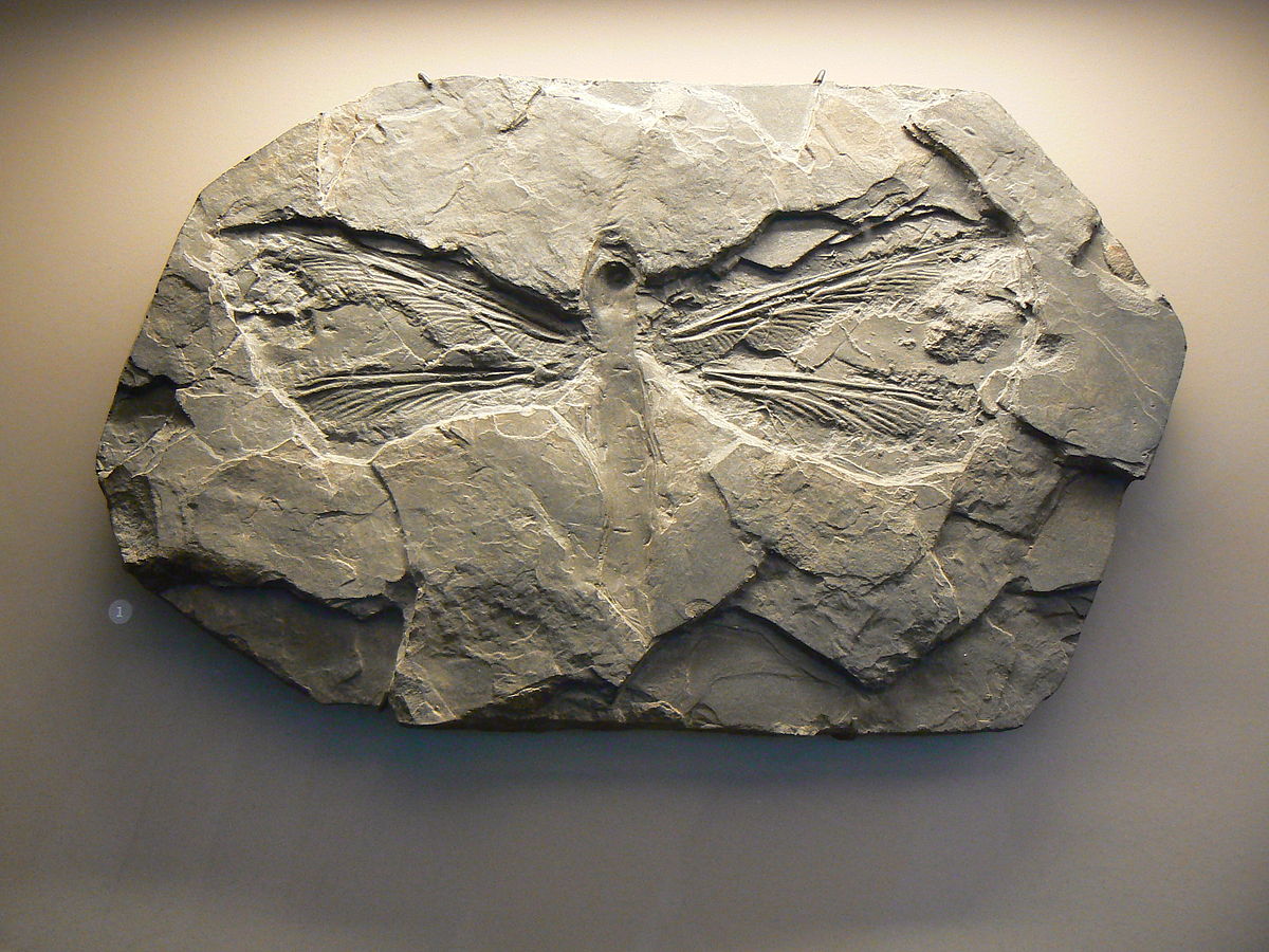
Creative Commons Attribution-Share Alike 3.0 Unported, 2.5 Generic, 2.0 Generic and 1.0 Generic license.
That’s a dragonfly the size of a hawk. Its wingspan is 28 inches (70 cm). It could never survive today, but during the Carboniferous, with an atmosphere of 35% oxygen, such a huge insect was plausible. Other examples of giant arthropods include Arthopleura and Megarachne.
Isotopes
Isotopes are atoms of a given element that vary in their weight. Atoms are made of protons, neutrons, and electrons. The number of protons in an atom determine its identity as an element. For instance, all oxygen atoms have eight protons. All carbon atoms have six protons. Usually, the number of protons (which carry a positive charge) is matched by the number of electrons (which carry a negative charge). This balance makes the atom electrically neutral. If there are more protons than neutrons, the atom is a cation. If there are more electrons than protons, it makes it an anion. We’ll ignore ions for the present discussion.
It’s the number of neutrons that matters for determining isotopic identity. In addition to its six protons, a given atom of carbon can contain six neutrons, seven neutrons, or eight neutrons. When you add the number or protons to the number of neutrons, you get the atomic mass of that atom.
6+6=12
6+7=13
6+8=14
So that means carbon atoms come in three isotopic varieties: 12C, 13C, and 14C. You’ve probably heard of 14C (carbon-14) as the basis of dating recent organic remains, such as wood, bone, or tissue. It is radioactive, meaning the atom is unstable. Eight is one neutron too many, and the forces that hold the atom together are incapable of maintaining its structure over the geological long-term. As a result, it’s not useful to us for the current discussion. It’s also a tiny amount of all carbon, about one part in a thousand. So let’s set 14C aside and focus now on 12C and 13C instead.
12C and 13C are not radioactive; the forces that hold their atoms together are durable over geological spans of time. Hence, we call them “stable” isotopes. 12C is “light carbon.” 13C is “heavy carbon.” Most carbon atoms are the lightweight kind, 12C. It makes up about 99% of all carbon atoms. But there is also a measurable amount of heavy 13C, comprising about 1% of all carbon on Earth.
It turns out that various natural processes separate light carbon from heavy carbon. These acts of separation, called isotope fractionation, enrich some parts of the Earth system in 12C, while depleting other parts. For instance, photosynthesizing plants prefer 12C-based CO2 molecules, meaning that plants (and the animals that eat the plants) are enriched in 12C, but that act of removing 12C from the atmosphere makes it relatively depleted in 12C. Or if you consider it from the perspective of the less-common 13C atoms, then it’s the other way around: life is the reservoir that’s depleted in heavy carbon, and the atmosphere is enriched in heavy carbon. The ratio between these two isotopes is something we use as an indicator of past conditions on Earth, such as its climate. The ratio of 12C and 13C gets skewed between the major reservoirs in the Earth system as climate shifts. The same is true of heavy oxygen and light oxygen (16O vs. 18O), or light hydrogen and heavy hydrogen (1H vs 2H, the latter of which is also called D for “deuterium”). Critically, with all these isotopes, we can measure that skew.
This video discusses three different elements (hydrogen, oxygen, and carbon) in terms of natural fractionation of their isotopes, and relates that fractionation to Earth’s prevailing climate:
Because plants prefer 12C over 13C, during times when there are high rates of carbon burial happening on Earth, much of the 12C ends up underground, being converted to coal, oil, or natural gas. That means the atmosphere will be relatively enriched in 13C instead. Because the ocean exchanges gases with the atmosphere, the waters of the ocean will also be enriched in 13C instead of 12C.
When climate is cool, there is less energy available to drive evaporation, so ocean water tends to be enriched in heavier isotopes: water molecules containing deuterium or 18O. Evaporated water molecules are more likely to be isotopically lighter, and so will the precipitation that they drop. During ice ages, the snow that falls to make glacial ice will be a reservoir of isotopically lightweight water, both in terms of hydrogen and oxygen.
Fossil fuels
Buried carbon does not necessarily stay buried. Our species has found it useful to extract carbon-rich gas, liquid, and solid compounds from the crust and set them on fire. By oxidizing that carbon, we release energy originally bound up in chemical bonds as much as ~350 million years ago. We refer here to and coal, petroleum, and natural gas: the “fossil fuels.” They get this name because all the carbon in each fuel came originally from living things extracting CO2 from the atmosphere. Fossil fuels would not exist without life. (Fossils are the remains of ancient life.) Specifically, ancient bog and swamp plants were the precursors for coal, and ancient phytoplankton were the precursors for petroleum and natural gas.
Coal
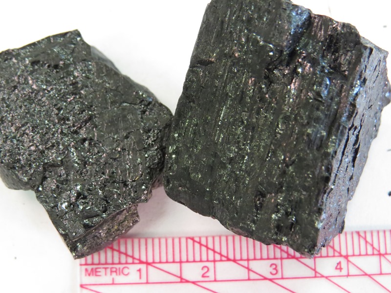
Ralph & Cheryl Dawes photo.
Coal is a solid fossil fuel that forms from compressed plant matter called peat. Frequently coal layers (“seams”) still retain the impressions of leaves, stems, seeds, spores, and other botanical details. Coal comes in several “grades” that reflect varying degrees of compression. The lowest grade is lignite (brown coal), which is just a step up from peat, the original mix of plant bits. If it is more compressed still, it will become bituminous coal. And the highest grade of coal, anthracite, forms only when a coal seam is subject to metamorphism under the influence of mountain-building.
Callan Bentley photo.
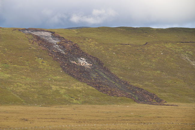
The plants that are the progenitor of coal live on the land, in wet, aquatic, or swampy settings. It’s traditional to think of coal as coming from swamps, since swamp water is usually stagnant, and thus poorly oxygenated. Carbon-rich plant fragments falling into that water are therefore more likely to avoid oxygenation long enough to be buried. The rate of new carbon being added as plants shed debris outstrips the rate at which oxygen diffuses across the calm surface of the water.
But peat can also form in cool, wet climates such as Ireland or Scotland. There, a layer of vegetation clings to the topography of the land. The damp weather means that sphagnum and heather, the main peat-building vegetation, grow on slopes and hilltops as well as in the valley bottoms, with underlying peat layers averaging a meter or two thick. The entire landscape is essentially blanketed in bog. It grows upward at about 1 cm/year.
Oil
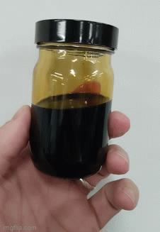
Callan Bentley GIF.
Oil has a different origin story. Here, the photosynthesis was conducted by marine or lake algae, phytoplankton floating as single-celled organisms in the uppermost, sunlit portion of the water column. When they died, their bodies rained down to the bottom. This transferred the carbon they contained to the dark depths. Often, the bottoms of lakes or the ocean have far less dissolved oxygen than waters closer to the surface. As a result, carbon entering these anoxic waters tends to be buried before it can oxidize. As with swamp coal, it’s a case of the carbon burial rate exceeding the flow of dissolved oxygen to the same place.
Once buried, the algae have to be warmed up to a critical temperature – about 100°C, the temperature of a freshly made espresso. If it’s too cold, their little dead cells won’t transform into petroleum. If it’s too hot, the mixture will turn into natural gas (described below) and graphite. The temperature has to be just right.
USGS image.
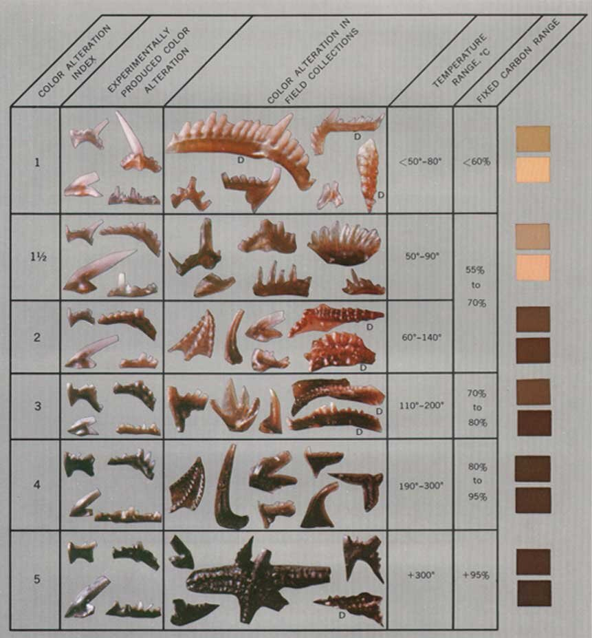
Interestingly, one way geologists can make a quick but accurate assessment of the temperature to which potentially-oil-bearing rocks have been warmed is by examining fossils. Specifically, the spiky “elements” of the conodont animal. These are made of hydroxylapatite, a phosphate mineral. The key thing to know about hydroxylapatite is that it changes color when heated, like a piece of toast. Geologist Anita Harris developed a vital tool with the Conodont Alteration Index, a 6-point color scale that uses the various “toastings” of conodonts to see if their host rocks warmed up to the appropriate temperature for oil generation.
Conodonts can then be collected from numerous sites in a region, their color assessed using the Index, and then the presence of each color can be contoured. Here’s an example for the sedimentary strata of the Appalachian Plateaus + the Valley & Ridge provinces:
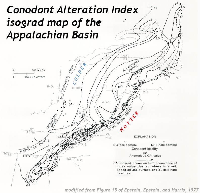
Modified from a USGS figure.
Once produced, oil must migrate to a spot where it can collect in amounts where humans will find it economically worthwhile to drill it out and extract it. There are plenty of places where oil naturally seeps out at Earth’s surface, such as the legendary tar pits of Rancho La Brea in Los Angeles, California.
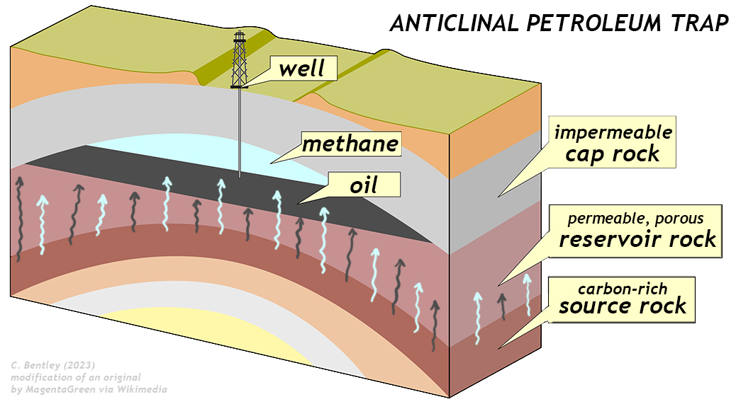
C.Bentley modification of an original diagram by GreenMagenta via Wikimedia.
But the oil you burn in your automobile found a stable residence underground in some variety of subterranean oil trap. These have various shapes due to various geological circumstances, but one of the easiest to grasp is that of an anticline. If the arch-like shape of an anticline consists of a stack of layers with carbonaceous source rocks at the bottom (such as black shale), impermeable cap rock strata (such as shale) at the top, and a spongey reservoir layer (such as sandstone) in between, that makes for an ideal petroleum trap. Petroleum geologists are charged with finding these traps and directing the company’s engineers to tap into them.
Natural gas
Modified from a Terry Engelder photo.
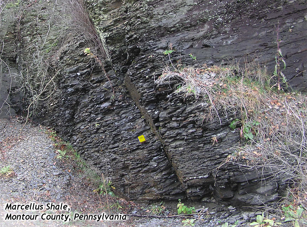
Our third and final fossil fuel is neither a solid like coal, nor a liquid like oil. Instead, it’s a mixture of gases, principally methane (CH4). Like oil, its progenitor is phytoplankton. While these algae live, they photosynthesize. When they die, their bodies rain down into anoxic deep waters, imparting a high carbon content to the sediments deposited there. Typically, the resulting rock is a black shale.
Black shales are more common in the geologic record during times of sluggish ocean circulation or widespread stagnation, such as the end-Permian or the mid-Cretaceous. Black shales can also be deposited in lakes; they are not necessarily marine in origin.
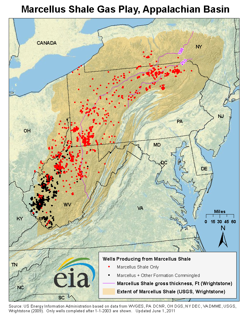
US Energy Information Administration map.
The Marcellus Shale of the Appalachians and the Bakken Shale of the Dakotas are both Devonian-aged black shales with lots of natural gas trapped inside them. In the past decade, the advent of horizontal drilling has allowed fossil fuel companies to drill into these shales and intentionally shatter them, allowing the gas to flow out, up the drill hole, where it can be collected, transported, and sold. The shattering process is achieved by (a) injecting fluids under very high pressures, along with (b) sand, which props open the fractured shale once the cracks open up. This process is called hydraulic fracturing, or “fracking.”
Natural gas is also produced in coal seams. This variety is referred to as “coal-bed methane.” Coal miners have been very conscious of coal-bed methane since coal mining began – because it is invisible gaseous reduced carbon, one spark from mining equipment could trigger an explosion. Far too many miners lost their lives to this hazard. They called it (and any other inflammable gas) “firedamp.”
Anthropogenic climate change
Because of the rich energy content of fossil fuels, humans have gotten in the habit of burning them, and depending intensely on the burning. The modern global economy and the lifestyles of us modern humans are powered in large part by the combustion of fossil fuel — solids, liquids, and gases that derive their energy content from sunlight that shone on Earth tens to hundreds of millions of years ago. As plants do with oxygen waste, we toss our CO2 waste into the atmosphere. Because it’s invisible, we’ve been able to ignore it for a long time. Out of sight, out of mind.
CO2 rise
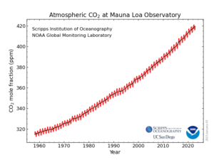
Scripps / NOAA graph.
Since humanity began burning fossil fuels in earnest (the start of the Industrial Revolution), CO2 levels have increased in the atmosphere of our world. The seasonal signal of photosynthesis is still there, but every year, CO2 ends up at a higher level than the previous year. From a pre-Industrial level of ~280 parts per million (ppm) to the current ~420 ppm, it has increased by about 50%.
It would have been an even larger increase, had not the Earth system been so intimately inter-connected. Much of the CO2 that humanity has emitted through the burning of fossil fuels has been re-extracted from the atmosphere: some has been taken out by plants doing photosynthesis more efficiently, and some has been soaked up by the oceans.
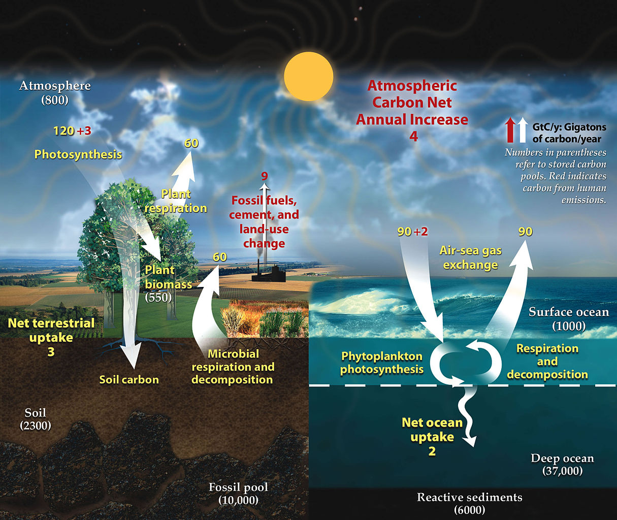
NASA graphic.
Estimates of the flow of carbon between reservoirs in the Earth system suggest that human activities release about nine billion tons (gigatons) of carbon into the atmosphere per year, of which three is then pulled out again by plant photosynthesis, and two is dissolved in the oceans. That leaves a net atmospheric gain of four gigatons per year. Examine the graphic at left to explore the complexities of carbon fluxes between reservoirs, but follow the red numbers, which show the changes that result from the human economy’s dependence on burning ancient trees and algae. This imbalance is why the graph above shows a relentless climb: the rates of carbon absorption can’t match the rates of carbon emission.
Oceanographers are well aware of one of the consequences of this natural carbon sequestration: those extra two gigatons of carbon soaked into the oceans each year produce carbonic acid, which is making the ocean overall more acidic. Already surface ocean pH has dropped by 0.1 unit, with a forecast total of -0.7 pH units change over the next 750 years. This potentially has enormous effects for the viability of life in the oceans. Many of our greatest episodes of mass extinction are correlated with times of intense ocean acidification.
But the bigger issue is probably global warming. Because of the selective transparency of the CO2 molecule, the higher level of this greenhouse gas has resulted in Earth retaining more energy than previously. This has caused the average global temperature to increase.
NASA animation of NASA data.
There are many consequences of this change in the planet’s climate, including: melting glacial ice and permafrost, rising sea levels, intensification of tropical storms, increasing desertification, and a spur to the migration of species toward more pole-ward latitudes and higher elevations. It is an interesting time to be alive and scientifically aware on planet Earth.
O2 fall
There is another aspect of the burning of fossil fuels which is also noteworthy. The basic combustion reaction of C + O2 → CO2 generates CO2 of course, but it also consumes O2. For every atom of carbon we oxidize to power our energy grid or heat our homes or propel our vehicles, we lose one molecule of free oxygen from the atmosphere. Thus, as the past six decades of measurements show a rise in CO2, we should also expect a commensurate decline in O2.
Indeed, that is what we have observed:
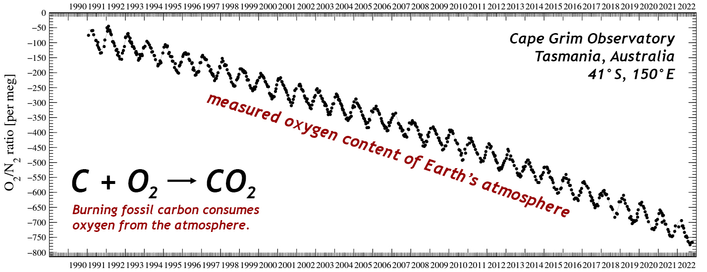
Graph by Scripps O2 program, annotated by C. Bentley.
At first glance, this graph might seem alarming to readers who breathe oxygen, but remember that this is a parts-per-million level decline in a very large reservoir of oxygen: ~21%. It represents a drop of a few ten-thousandths of the total amount of oxygen. So you don’t have to worry about running out of breathable air. We will exhaust our supply of fossil fuels long before atmospheric oxygen levels change by even 1%.
Instead, save your worrying for the impacts of global warming.
Further reading
Wally Broecker, 1996. “Et tu, O2?” 21stC, Columbia University.
Ken Caldeira and Michael Wickett, 2003. “Anthropogenic carbon and ocean pH,” Nature 425, p.365. https://doi.org/10.1038/425365a
Anita Epstein, Jack Epstein, and Leonard Harris, 1977. “Conodont color alteration — an index to organic metamorphism.” USGS Professional Paper 995. 27 pages.
Ian Glasspool and Robert Gastaldo, 2022. “A baptism by fire: fossil charcoal from eastern Euramerica reveals the earliest (Homerian) terrestrial biota evolved in a flammable world,” Journal of the Geological Society pre-print. Accessed online 14 January 2023.
Iman Gosh, 2021. “All the Biomass of Earth, in One Graphic,” Visual Capitalist. (20 August 2021) Retrieved 10 January 2023.
Elizabeth Kolbert, 2006. “The Darkening Sea,” The New Yorker. November 20, 2006, p.66.
Museum of the Earth, 2023. “Anita Harris,” Daring to Dig Paleontologist Profiles. Retrieved 12 January 2023.
Holly Riebeek, 2011. “The Carbon Cycle,” NASA’s Earth Observatory. Retrieved 12 January 2023.
A.A. Venn, J.E. Loram, A.E. Douglas, “Photosynthetic symbioses in animals,” Journal of Experimental Botany, Volume 59, Issue 5, March 2008, Pages 1069–1080, https://doi.org/10.1093/jxb/erm328