LEARNING OBJECTIVES
After reading this chapter, students should be able to:
- Describe the difference between a tectonic plate and a tectonic boundary
- Summarize the key geologic characteristics of each of the three major tectonic boundaries (transform, divergent, and convergent)
- Interpret the geologic evidence of historical plate interactions
- Summarize driving forces of plate tectonic activity
- Explain Wilson cycles
Introduction
In the late 1960s and early 1970s, geoscientific consensus gelled around an intriguing idea: that many different observations about our planet could be explained with a single model of Earth dynamics. The idea of “plate tectonics” put together old ideas about continental drift with new data showing seafloor spreading. The new theory was a revolutionary idea that made the distribution of volcanoes, earthquakes, continents, and topography make sense in a way that no idea had achieved before. Fifty years of additional data and testing have confirmed plate tectonics as the key idea in modern geology.
Plates
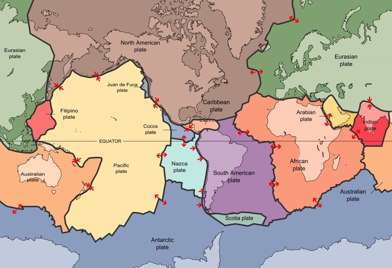
Public domain from Wikipedia.
Earth’s outermost rocky surface, the lithosphere, is broken into a series of big curvitabular pieces that move about relative to each other. Depending on how you count them, there are about 15 of these slabby pieces. We call them plates, and they range from about 50 km to 280 km thick and are mostly stiff upper mantle, but the upper part of each consists of crust. As humans, this is the part we can see and explore. The crust comes in one of two varieties: continental crust or oceanic crust. Together, the crust and the upper mantle comprise the lithosphere.
Oceanic lithosphere is a lot thinner and denser than the continental lithosphere. On average, the continental crust tends to be about 30 km thick, but it can get to be close to 100 km thick under new mountain belts, and is thinner beneath rift zones, weak spots where the crust is stretching. The oceanic crust is much thinner, around 10 km thick on average. It’s thinnest beneath oceanic ridges, prominent features that rise from the seafloor and wrap around the planet through the ocean basins like seams on a baseball. The mantle portion of the lithosphere is the same composition beneath the continents and oceanic crust. It differs from the rest of the mantle not so much in its composition but in the way that it behaves: it rides around with the overlying crust as a more or less stiff unit.
Let us first consider the position of the plates in terms of the planet’s layered structure. The lithosphere sits atop the asthenosphere, which contrasts in its behavior. The asthenosphere is a weak layer in the mantle that is mostly solid but perhaps 0.5% molten. This tiny amount of melt (99.5% solid) dramatically lowers the strength of the asthenosphere. The prefix asthenos means “weak” in Greek. Movement in the asthenosphere contributes to the motion of the lithospheric plates.
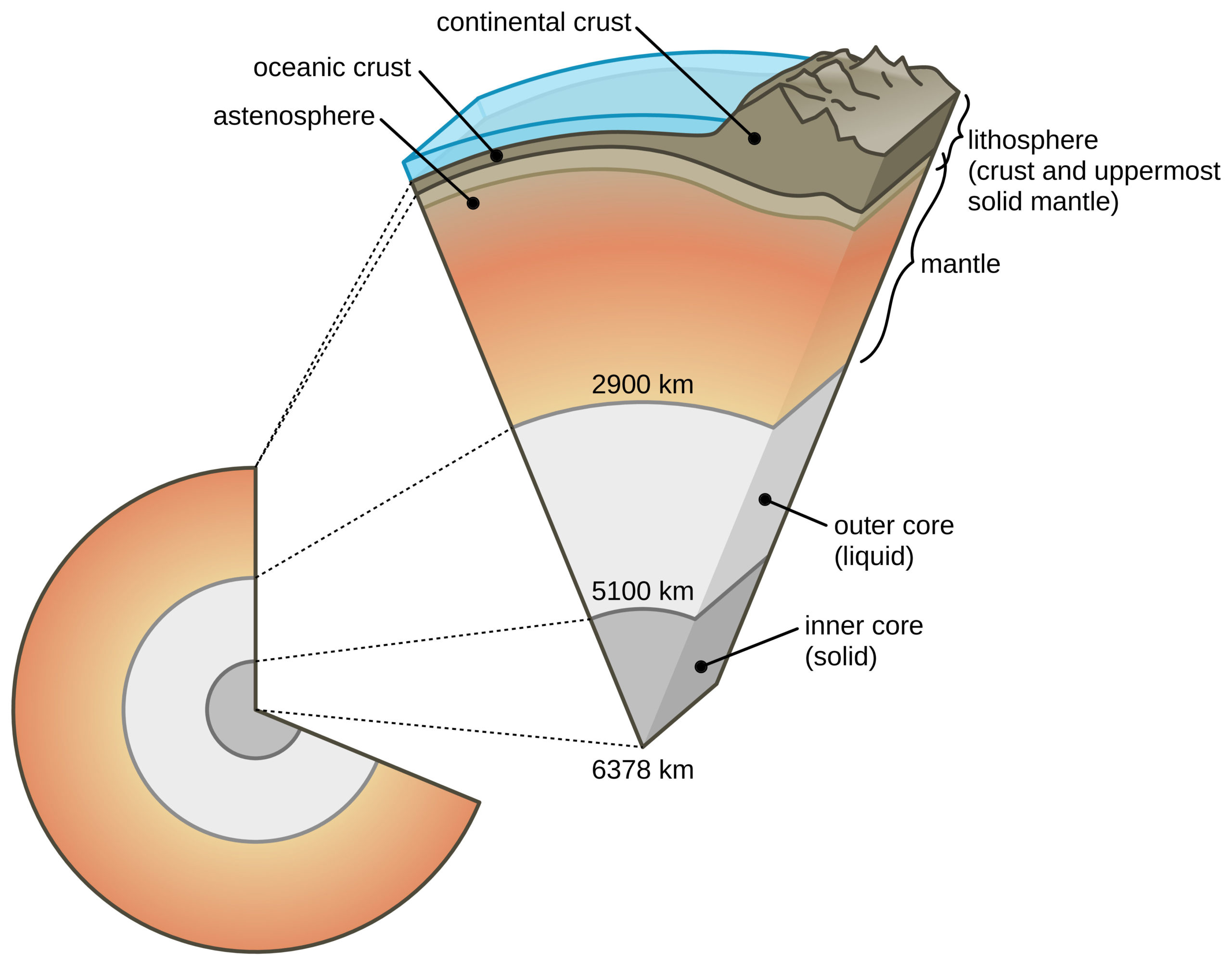
Image credit: U.S. Geological Survey.
Beneath the asthenosphere is the lower mantle, and beneath that is the core. The core consists of an inner solid portion and an outer liquid portion. Both are made of an alloy that is mostly iron, plus ~5% nickel and some sulfur. The outer core convects, and in so doing generates a powerful magnetic field that extends through the surrounding shell of rock and out into space.
Above the lithosphere are the oceans and/or atmosphere. These sit higher than the rocky plates, since they are less dense. Though they sit at the same level, continental lithosphere is more buoyant than oceanic lithosphere since the continental crust is made of less dense rock than the oceanic crust. It is a situation akin to a Zodiac raft and a surfboard both floating on the surface of a lake. The ordered layering of atmosphere, ocean, crust, mantle, and core is a reflection of a mature planet, that has differentiated into distinct horizons of varying density:
| Atmosphere | 0.001 g/cm3 |
| Ocean water | 1.0 g/cm3 |
| Continental crust or oceanic crust | 2.7 g/cm3 or 2.9 g/cm3 |
| Mantle | 3.3 g/cm3 |
| Core | 11 g/cm3 |
As far as their size goes, the plates can be large or small. The largest plates are the Eurasian Plate and the Pacific Plate. The smallest is harder to define. The Juan de Fuca Plate is only 250,000 km2, a relatively tiny slab in the eastern Pacific Ocean, but there are even smaller “microplates” of oceanic lithosphere between the Pacific and Nazca Plates, too. The smallest plate consisting primarily of continental lithosphere is the Arabian Plate, at 5,000,000 km2. Some consider the crust beneath California’s Sierra Nevada and Great Central Valley to be a microplate, one that has foundered a bit to the west.
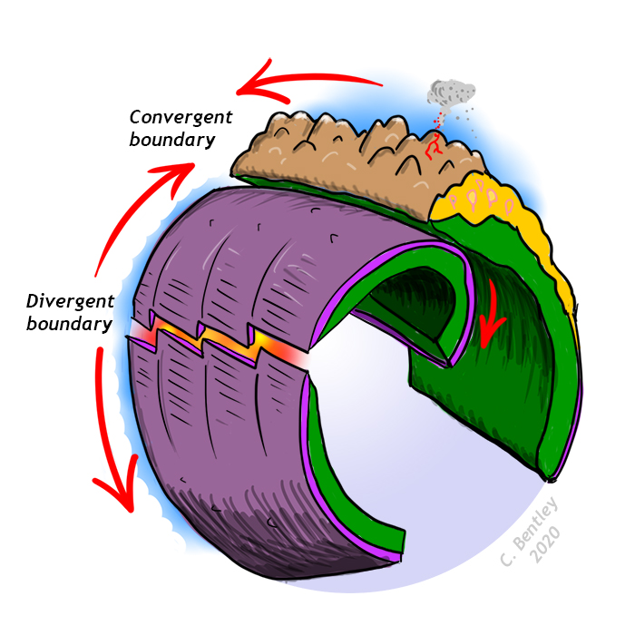
Drawing by Callan Bentley.
The shape of the plates is kind of like fragments of an eggshell, or pieces of orange peel: they are both “slab like” or tabular in some senses, but also curved, as fragmental pieces of an overall spheroidal shell. There’s no perfect word to describe such a shape, but perhaps “curvitabular” conveys a sense of it.
In map view, the shape of these curvitabular plates varies tremendously. Their edges can be more or less straight lines, arc-like curves, or zigzag-like patterns resembling irregular stair steps. They can even be broad, diffuse zones rather than crisp, well defined boundaries. And each of these boundary shapes is shared with another plate. Each of these shapes conveys information about the relative sense of motion of the plate movement.
Did I get it?
Tectonics
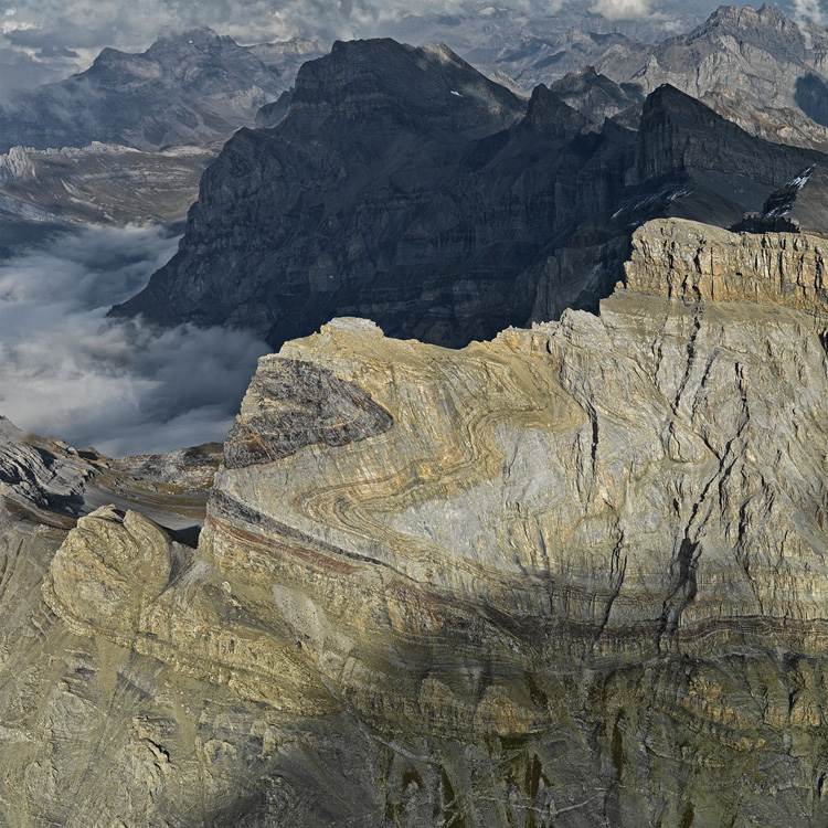
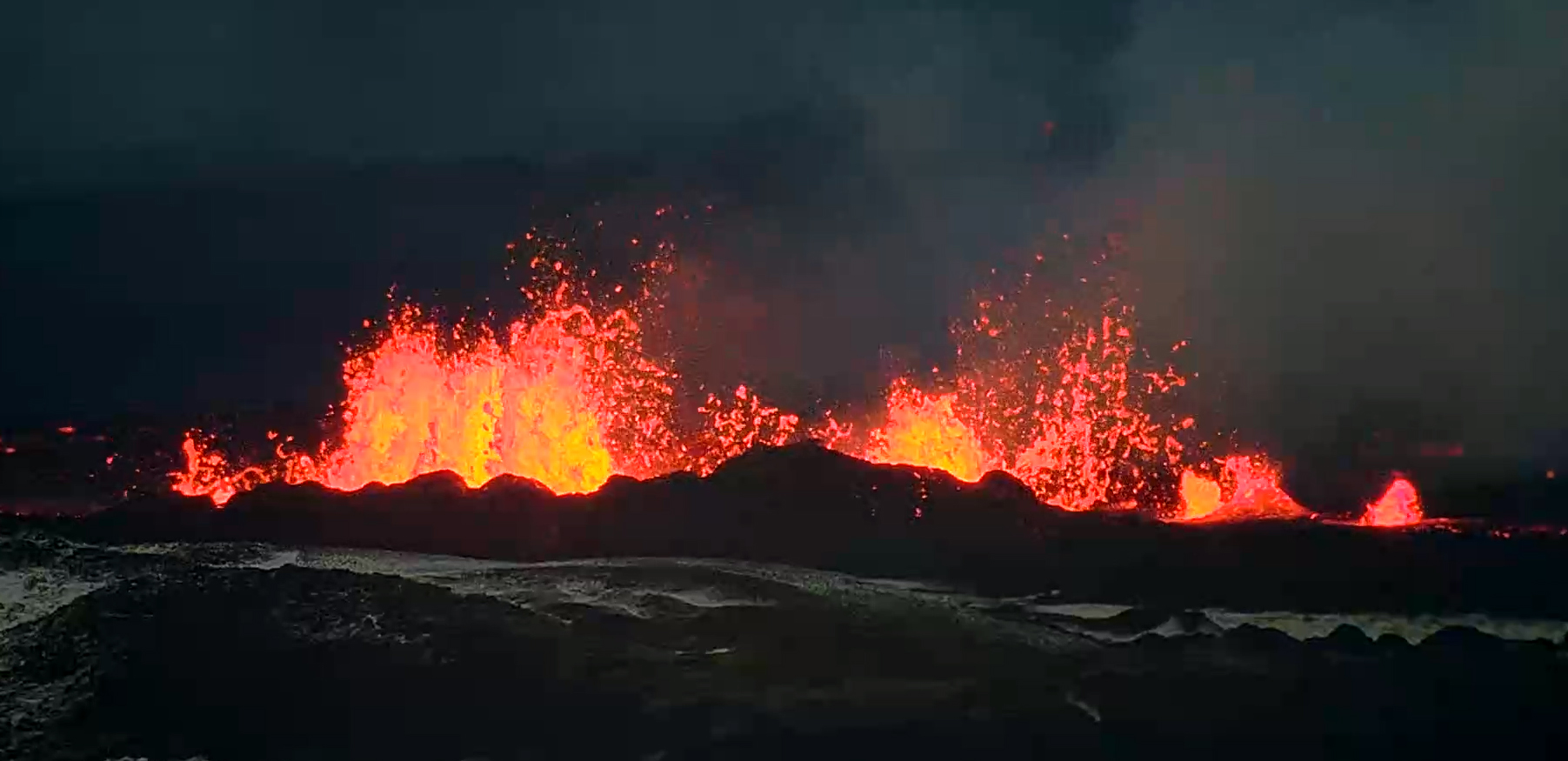
Photograph by Bernhard Edmaier; reproduced with permission.
Much of the attention we devote to lithospheric plates is focused on their boundaries, where much of their dynamic action takes place. That this dynamic action is located at the plate boundaries was the insight that led to the second part of the name: tectonics. This word means action in the sense of “building” or “constructing” things – specifically building belts of mountains. The root word is again Greek, and tektonikos means “building” or “making.”
So in literal translation, the phrase plate tectonics means “building [mountain belts] using plates” but in current usage by scientists, the theory of plate tectonics covers much more than just mountains. It also encompasses our understanding of volcanic island arcs, ocean basins, earthquake locations, and disparate lines of evidence that document the long-term motion of lithospheric plates.
Boundaries
By and large, the action of plate tectonics happens at the edges of plates, where they meet their neighbors. These plate boundaries come in three principal varieties, determined by the relative motion between the neighboring plates. Are they coming together, moving apart, or simply grinding past one another in opposite directions? We call these situations convergent, divergent, and transform. The dynamics of their relative motion end up determining which suite of geological processes and phenomena will result.
Did I get it?
Transform boundaries
Callan Bentley photo.
Transform boundaries are the simplest kind of plate boundary. At a transform boundary, new lithosphere is neither created nor destroyed. Instead, the two plates slide past one another in opposite directions, grinding slowly along a fault zone. Friction acts to restrain the plates’ motion. Moments when the friction is overcome — and the plates slip rapidly and violently — are earthquakes. Earthquakes are the main geological phenomenon to be aware of at transform boundaries, but the earthquakes there are distinct in that they are relatively shallow (20 km deep or less), and range in magnitude between small and large (~M7.5 at the most), but they are never huge, like the largest quakes that can occur (~M9) at convergent boundaries. Rock is weaker under shear than under compression, so less stress builds up at transform boundaries.
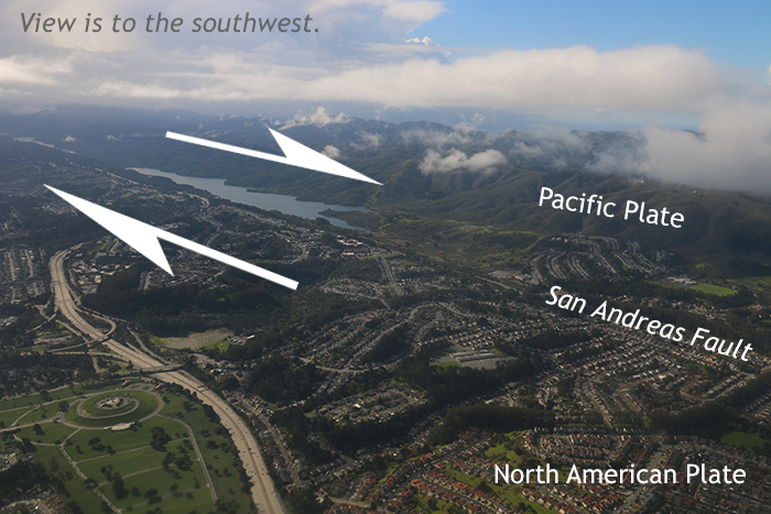
Transform boundaries can be recognized by offset features that cross the plate boundary fault zone such as bodies of rock, landscape features such as stream valleys, or human-built structures such as roads and fences. The faults that form on transform boundaries are either right-lateral or left-lateral. The San Andreas Fault in California is right-lateral: from the perspective of the Pacific Plate, the North American Plate is moving to the right. From the perspective of the North American Plate, the Pacific Plate is moving to the right.

Landsat image from NASA.
It doesn’t matter which side of the fault you stand on; the apparent motion of the opposite side is to the right. The North Anatolian Fault in Turkey is another example of a right lateral fault, with the Anatolian Plate moving west relative to the Eurasian Plate. The North American Plate’s southern margin is a left-lateral transform boundary with the Caribbean Plate. This boundary is distributed across two major faults, the Enriquillo-Plaintain Fault and the Septentrional/Oriente Fault.
Faults are are zones where rock is broken. Because crushed-up, pulverized rock weathers and erodes more rapidly than unbroken rock, the landscape of transform boundaries frequently shows linear features parallel to the trace of the fault zone: straight valleys and coastlines, elongated peninsulas, and bays.
The deeper record of this crushing can be exposed much later at Earth’s surface. When historical geologists find a zone of fault breccia, they can deduce that they are looking at a shallow fault. Deeper in the crust, the rocks are hotter and under more confining pressure, and they deform in a different fashion as a result. Instead of fracturing, the minerals flow in the solid state, producing the smeared-out rock called mylonite. Compare the wispy, foliated texture of a mylonite with the chunky texture of a fault breccia here:
Callan Bentley photo.
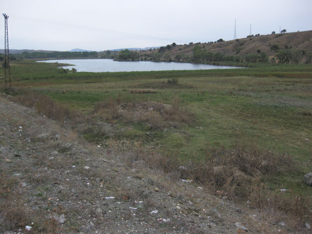
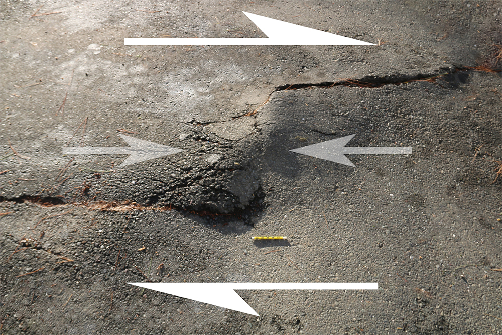
In places where the trace of the faults on a transform boundary are not parallel to the plates’ motion, there can be localized areas of compression or tension. When the orientation of the fault trace weaves a bit to the left or right, we call it a stepover. A right step in a right-lateral transform fault will create a zone of extension. This could manifest as a sag pond if it is small, or if bigger, it will make a larger trough like the Salton Sea or the Sea of Marmara. A left step in a right-lateral fault will generate a zone of compression, forcing rock upward into a pressure ridge. Pressure ridges can be small enough to see in a parking lot pavement, or the size of mountains.
Callan Bentley photo.
Continental transform boundaries are striking, but far more common are examples of transform faults in the oceanic lithosphere. Between segments of oceanic ridge on the seafloor are zones where the plates slide past one another. These are oceanic transform faults, and they are a key feature of overall divergent boundaries in our planet’s ocean basins. Together with the oceanic ridges you’ll learn about below, the create the distinctive zigzag shape to most oceanic divergent plate boundaries.
Did I get it?
Divergent boundaries
Divergent boundaries are sites where two plates move away from one another. In this extensional setting, normal faulting dominates, thinning the crust vertically while stretching it out laterally. Divergent boundaries come in two principal varieties that are relevant to historical geology: rift valleys in continental crust and oceanic ridges in oceanic crust.
Continental rifting
When a divergent boundary develops in continental crust, it has two consequences, one sedimentary and one igneous.
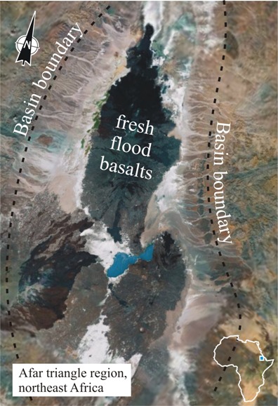
NASA photo, annotated by Callan Bentley.
The sedimentary consequence is most apparent where divergent boundaries occur in continental lithosphere. The normal faulting down-drops a block of crust, producing a graben or “rift valley.” The classic modern example is the Great Rift Valley of east Africa (pictured here).
The edge of the rift valley (the escarpment) is a site of high topographic relief, which encourages clastic sediment to drop downhill from the surrounding highlands into the rift valley. This sediment does not travel far, or for very long. As a consequence, it tends to be compositionally and texturally immature. Alluvial fans of poorly-sorted gravel flank the escarpment, smoothing out the highest relief areas. Finer grained sediment gets carried a bit further, and creates deposits of arkosic sand. Lakes accumulate in the lowest regions, furthest from the rift escarpment, growing salty as they evaporate.
A very similar situation can be seen in older, now-inactive rift valleys. For instance, the Culpeper Basin of central Virginia was an active site of rifting during the Triassic and Jurassic, as the supercontinent Pangaea was breaking apart and the Atlantic Ocean was first ‘being born.’
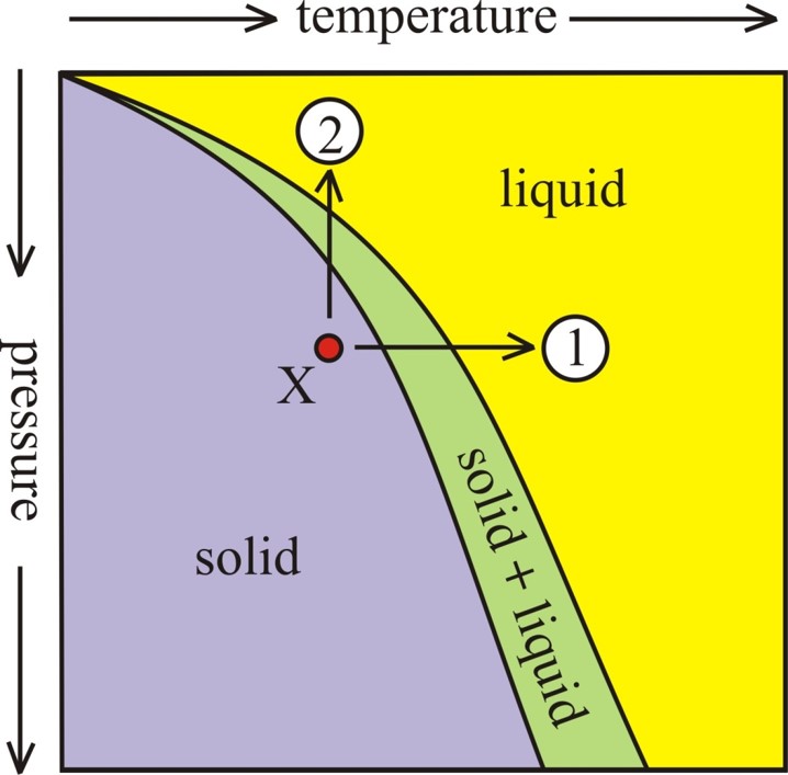
As far as igneous consequences of crustal thinning, consider the decompression of the underlying mantle. Already hot, the lowering of the confining pressure allows melting to occur without the addition of any new heat. Partial melting of ultramafic peridotite generates a mafic magma, which may rise to the surface to erupt as “floods” of low-viscosity basalt. This is plain as a half dozen large black patches in the satellite image here, showing the Afar Triangle region of northeastern Africa.
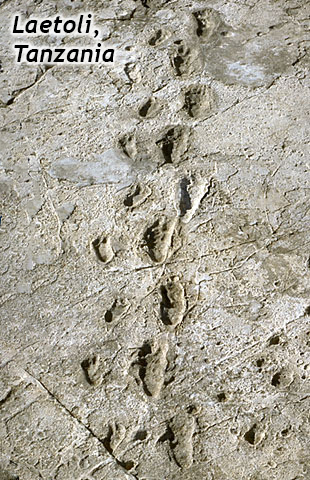
If the basaltic magma interacts with the crust on its ascent, it can transfer some of its heat and produce intermediate magmas, resulting in composite volcanoes such as Mt. Kenya, Mt. Kilimanjaro, or Mt. Meru. It was felsic ash erupted in the East Africa rift that preserved the footprints of two Australopithecines waking side by side at Laetoli, Tanzania, 3.2 million years ago.
Continental rifting is only the beginning of a divergent boundary however. Once the crust is sufficiently thinned, seafloor spreading takes over. This can be seen just north of East Africa, where a narrow body of oceanic crust separates Africa from Arabia. The Red Sea and the Gulf of Aden are just a bit more ‘tectonically mature’ than the Great Rift Valley. Here, the continental crust has fully broken into two discrete separate segments, diverging as Arabia moves to the northeast. New oceanic crust is filling the gap between them, a process called seafloor spreading.
Seafloor spreading
Callan Bentley diagram.
In seafloor spreading, decompression melting of the mantle produces mafic magma. This magma cools at various depths to produce new oceanic crust. When freshly minted, this oceanic crust makes a bathymetrically high feature on the seafloor, an oceanic ridge (also called a “mid-ocean ridge,” since many of them are in the middle of their host ocean basins).
No new heat needs to be added to mantle peridotite in order for it to melt via decompression: hot peridotite only needs to rise and experience lower pressures. Mantle convection brings warm rock upward, due to the warm rock’s low density. As it rises, it partially (not completely) melts beneath the oceanic ridge. This partial melting produces a magma that is mafic in composition from ultramafic source rocks.
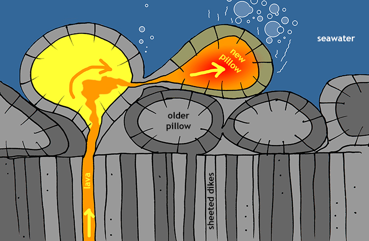
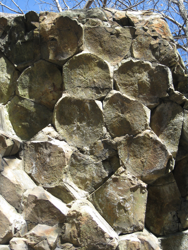
Callan Bentley cartoon.
As the plates diverge “overhead,” this mafic magma squirts into the crack between them. Some of the molten rock may make it all the way into the water and the bottom of the ocean, erupting to produce pillow basalts, while some magma cools rapidly and solidifies in the feeder crack itself, making a dike of basalt. Still more mafic magma cools slowly, deeper in the new oceanic crust, producing bodies of gabbro. This sequence of rock types is an ophiolite sequence – an important feature that we will return to again when we discuss convergent boundaries.
Animation by Tanya Atwater, UCSB.
Seafloor spreading happens at different rates in different ocean basins. The East Pacific Rise generates roughly twice as much new seafloor in a given amount of time as the Mid-Atlantic Ridge. At both oceanic ridges, sections of active divergences are offset along perpendicular segments of transform faulting, giving the plates’ edge a shape similar to a staircase. Because the mafic magma that cools to make oceanic crust cools to make magnetically-susceptible minerals such as magnetite, which will rotate into alignment with Earth’s magnetic field before the lava or magma around them solidifies. The generation of new oceanic crust through seafloor spreading therefore records changes in the polarity of Earth’s magnetic field (which happen due to changes in the core, and have nothing to do with the surface processes of plate tectonics).
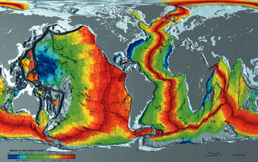
NOAA map.
Over time, the oceanic crust cools. As it cools, it becomes more dense. More dense rock sinks. The lithospheric mantle also builds out below, thickening through time to a maximum of around 100 km by the time it’s about 80 million years old. This adds substantial weight to the plate. This density-driven subsidence is combined with sedimentation atop the oceanic crust (adding more mass) to create the relatively smooth abyssal plains that floor most of the ocean basins around the world.
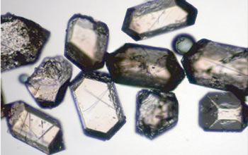
Photo: Michael John Cheadle, University of Wyoming, via NSF
We can determine the age of the seafloor by several methods: the first is direct dating of the crust via radioactive isotope decay systems in certain minerals. For instance, the gabbro of the deeper oceanic crust contains zircon crystals that host uranium→lead timekeepers. Another approach is analyzing the fossil content of sediments deposited on top of it. Index fossils in the deepest (oldest) sediment on a given patch of oceanic crust represent a time immediately after the new crust had formed due to volcanism. Finally, magnetostraigraphy of a stretch of oceanic crust can be measured and compared to the record of Earth’s magnetic polarity reversals from well-dated locations on the continents. Depending on the characteristics of the particular location, some of these methods may be more applicable than others. In those lucky locations where multiple methods can be applied, the different techniques can be used to corroborate each other’s age determinations.
Did I get it?
Convergent boundaries
When two plates are headed toward each other, we describe the situation as convergent. Depending on whether the leading edge of these two plates consists of oceanic lithosphere or continental lithosphere, several different situations can result.
Oceanic/Continental convergence
Public domain via Wikimedia.
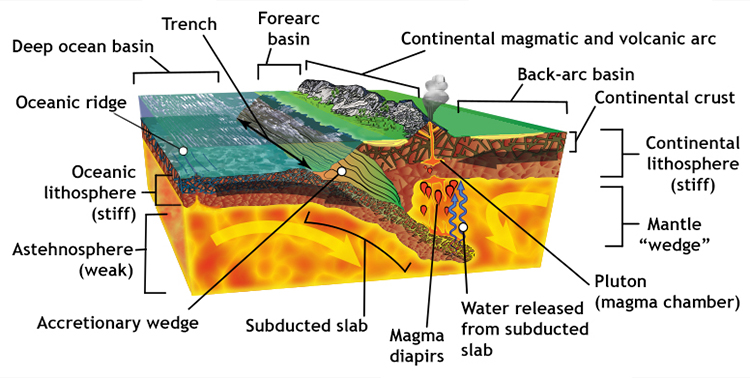
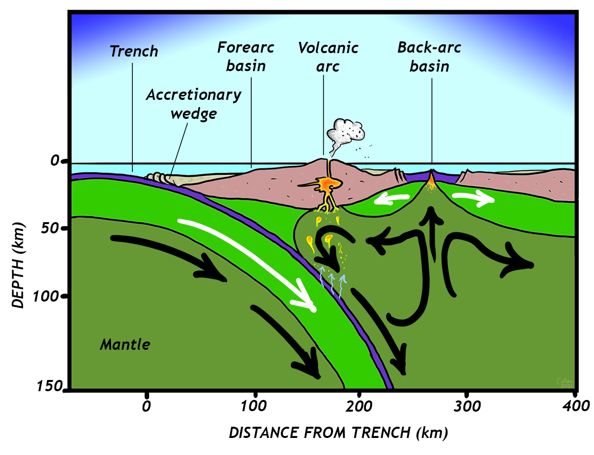
When oceanic lithosphere converges with a continent, subduction happens. Subduction is the situation when the plate of oceanic lithosphere descends down into the mantle beneath the plate bearing the continent. This subduction is marked by many phenomena: an oceanic trench marks the place where subduction begins, but earthquakes are generated all along the subduction zone to great depths beneath the overriding plate. The earthquakes at this megathrust fault can be among the largest known. At the trench, any sediment atop the plate may be scraped off, building up in a thick jumbled pile called an accretionary wedge. The accretionary wedge can also include volcanic rocks from seamounts and intrusions, as well as slices of the oceanic lithosphere itself.

Callan Bentley photo.
As it descends, the subducted plate releases water into the surrounding mantle. This water enables the melting of the ultramafic mantle rock, generating mafic magma. This magma rises and pools beneath the base of the continental crust, transferring its heat. The minerals of the continental crust tend to have lower melting temperatures, and so they melt, resulting in intermediate composition magmas, which continue to ascend through the crust. They may lodge at depth, crystallizing to make plutons and batholiths, or they may find their way to the surface, where they erupt as volcanoes. The development of a continental volcanic arc parallel to the trench is a sure indication of oceanic/continental convergence.
Callan Bentley diagram
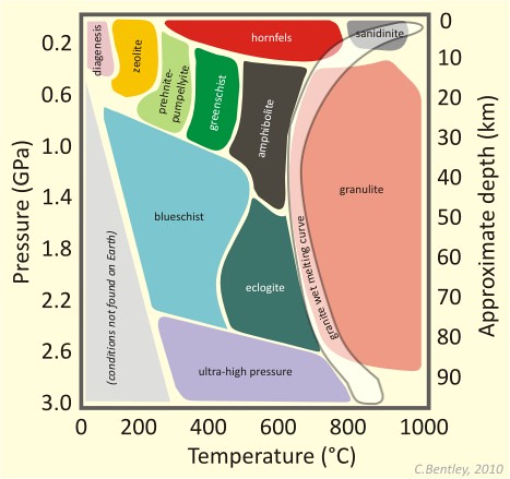
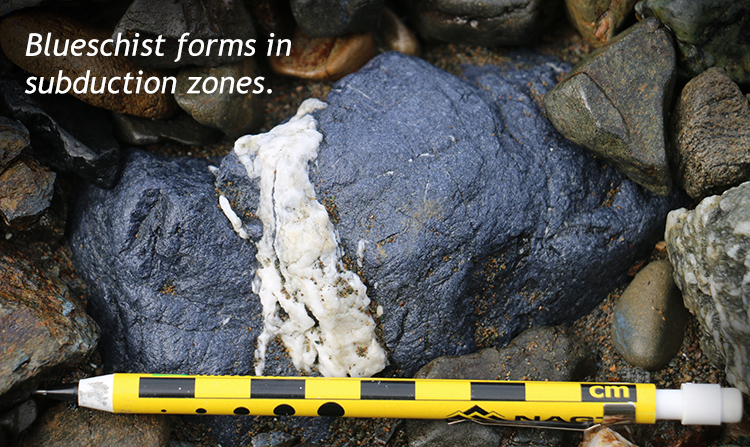
As the subducted plate descends, its rock experiences higher pressures and temperatures. These trigger metamorphosis. Specifically, subduction zones see rocks descending faster than they can warm up, and so they experience high pressures but relatively low temperatures. This results in blueschist and eclogite metamorphic facies.
Several places in the modern world are examples of this kind of plate boundary, including the Cascadia volcanic arc in the Pacific Northwest of the United States of America, but the classic example is the western edge of South America, where subduction of the Nazca Plate has resulted in the Andes volcanic arc as well as some of the largest earthquakes ever recorded.
Simkin, et al. (2006), USGS.
Ancient subduction zone complexes can be found in in many places that are no longer experiencing subduction: coastal California, central Turkey, western France, and the Cyclades of Greece are a few examples.
Oceanic/Oceanic convergence
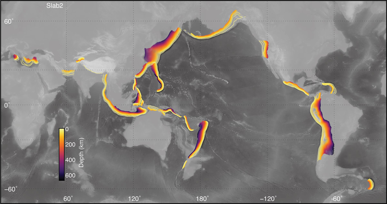
Gavin P. Hayes (USGS) map.
Volcanic island arcs result when two plates of oceanic lithosphere converge. As with the oceanic/continental situation, subduction results when one of the two plates descends beneath the other. Because they are both composed of the same rock types, the key variable is density based on age. Older oceanic lithosphere is colder oceanic lithosphere, and colder rock tends to be denser. For instance, in the western Pacific Ocean, ~200 Ma oceanic lithosphere of the Pacific Plate is subducting beneath ~20 Ma oceanic lithosphere of the Philippine Plate. In a match-up between old and young oceanic lithosphere, the young wins, and the old subducts. Because convergence with both continental lithosphere and young oceanic lithosphere “selects against” old oceanic lithosphere, there is very little of it still around. The oldest oceanic lithosphere left on this planet is Permian in age (~250 Ma), in the Mediterranean Sea.
So old oceanic lithosphere subducts, producing a trench and an accretionary wedge. Again the rock of the subducted slab undergoes dehydration reactions, releasing water into the mantle. This triggers melting of the mantle. The magma rises up to pierce through the overlying crust as a chain of volcanic islands. We call this a volcanic island arc.
In this overlay of the “Discovering Plate Boundaries” volcanology and topography maps, you can see this relationship plainly: in each location where we see a deep sea trench, it is paralleled by a volcanic island arc (line of red dots):
There is a strong coincidence of deep sea trenches and parallel belts of volcanoes.
Dale Sawyer’s “Discovering Plate Boundaries” maps.
Continental/Continental convergence
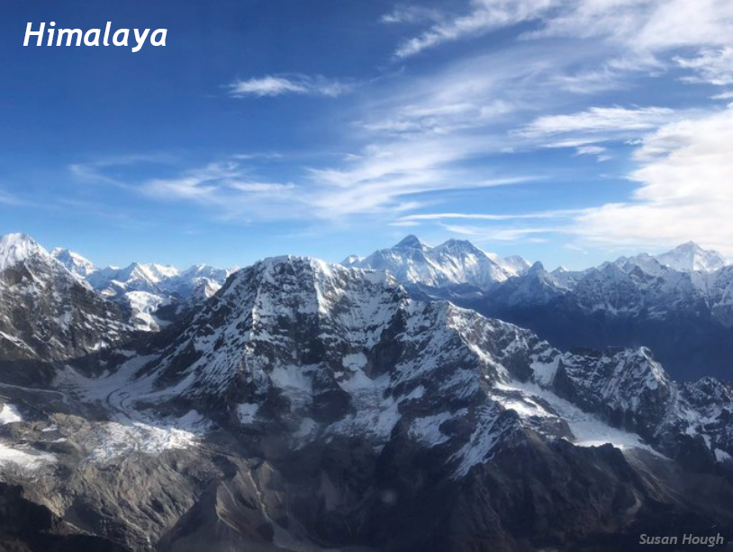
Photograph by Susan Hough; reproduced with permission.
The final circumstance that can happen at a convergent plate boundary is when all the oceanic lithosphere separating two continents has been subducted, and the two continents (formerly separated by an ocean basin) finally meet. Because of their buoyancy, the continents cannot subduct very far. Instead, they crumple upward into mountains. Deep below the plate boundary, the plate crumples too, thickening into a “keel” that extends downward. Extending all the way through the thickest lithosphere on the planet, this is a young collisional mountain belt. The act of forming a mountain belt is an orogeny (from the ancient Greek for “mountain making”).
The classic modern example of a collisional mountain belt is the Himalaya, which have been forming for the past ~40 million years where the Indo-Australian Plate is converging with the Eurasian Plate. Frequent large, shallow earthquakes mark this collisional zone, but there is no volcanism. (There is neither decompression melting nor slab dehydration occurring at a continent-continent collision.) There is probably partial melting occurring within the continental crust at the base of the mountains, making migmatite, but insufficient volumes of felsic magma are produced to generate volcanism.

Photograph by Stephanie Sparks; reproduced with permission.
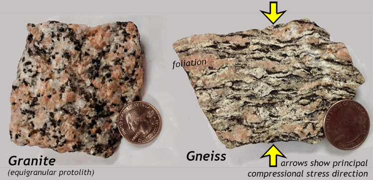
One consequence of this collisional mountain belt is regional metamorphism of the rock there. Where clay-rich protoliths encounter elevated temperatures and pressures at the roots of these mountains, metamorphic rocks such as phyllite, schist, and gneiss are generated. Porphyroblasts of metamorphic minerals such as chlorite, garnet, kyanite, staurolite, and sillimanite grow. Each of these minerals is a chemical manifestation of how atoms in Earth materials react to changing conditions. They represent a physical “snapshot” of pressure/temperature conditions when the rocks equilibrated to novel conditions within a mountain belt. Dating metamorphic minerals using mineral/isotope systems is one way we can determine when an episode of mountain-building happened.
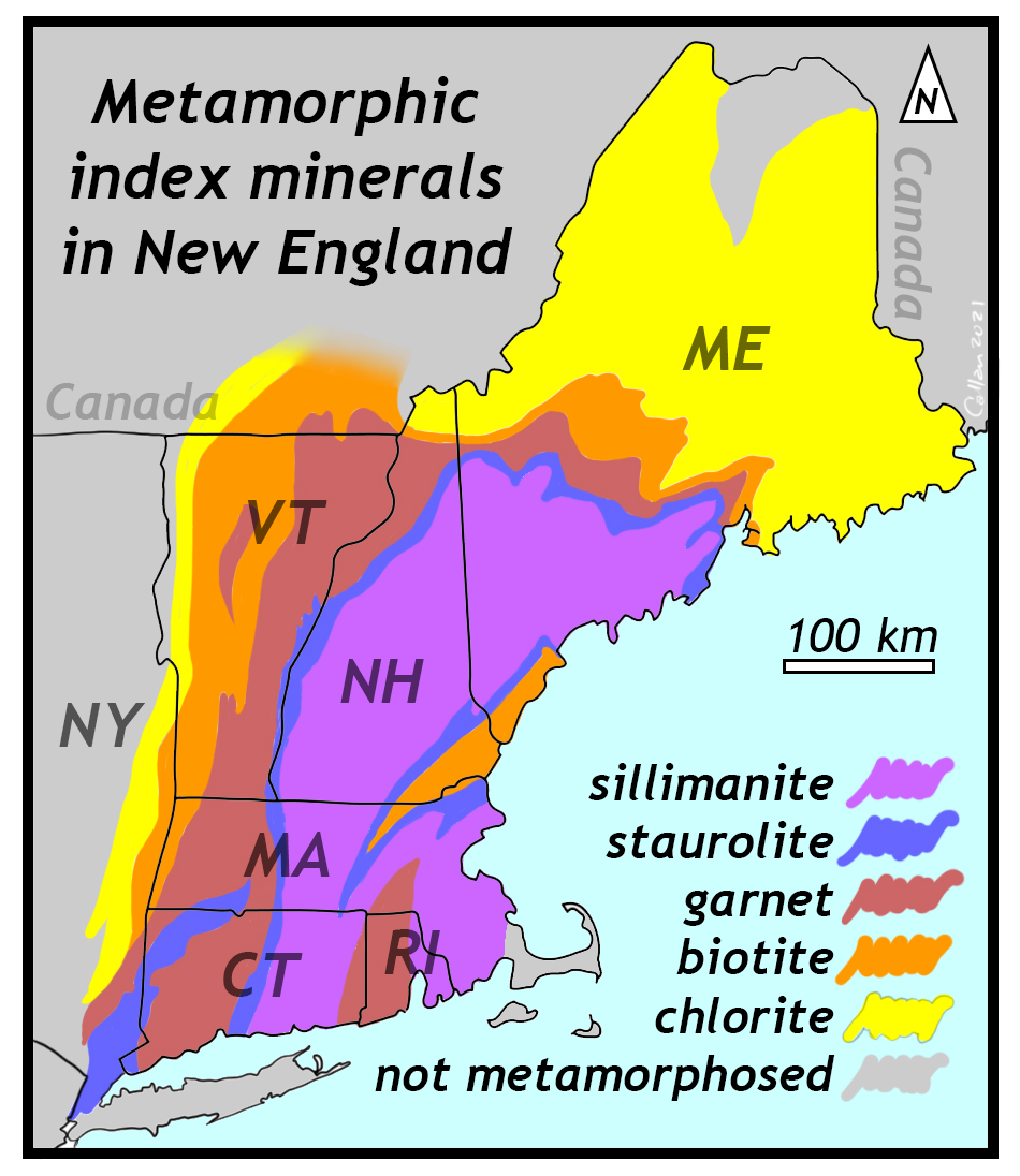
Callan Bentley graphic.
Even after the mountains’ topographic relief has been subdued by erosion, these metamorphic minerals serve as indications of the high temperatures and pressures at the roots of the mountain belt. For instance, in New England (northeastern United States), mountain building cooked and squished the rocks during the late Devonian Acadian Orogeny [LINK TO ACADIAN CASE STUDY]. A belt of high-grade metamorphic rocks stretches from south-central Connecticut north through central Massachusetts, where it splits. One of these sillimanite-bearing belts wraps around through eastern Massachusetts and south into Rhode Island, while the other widens at it trends north through New Hampshire and into southern Maine. The sillimanite zone is surrounded by zones of medium- and low-grade metamorphic rocks, as indicated by the minerals they bear as porphyroblasts. The staurolite didn’t get as metamorphosed as the sillimanite, but the garnet was even less metamorphosed. Biotite and chlorite mark lower grades of metamorphism yet. The sillimanite-bearing belt marks the rough position of the highest peaks when the mountains were freshly built.
Photograph by Jay Kaufman; reproduced with permission.
If the compressional stresses are strong, but the confining pressure and temperature are relatively low, rocks on the flanks of the mountain belt will be deformed through folding and thrust faulting. This zone of compressional deformation is distinct and pervasive in mountain belts across time and space. Fold and thrust belts form in pre-orogenic layered sedimentary and volcanic strata. Examples include the Pyrenees in Spain and France, the Cape Fold Belt in South Africa, the Valley & Ridge province of the Appalachians, the Ouachita Mountains in Arkansas, the Marathon Mountains in Texas, the Caledonides in Scandinavia, the Sevier Fold and Thrust Belt in the Rocky Mountains, the Damara Belt in Namibia, the Atlas and Anti-Atlas in Morocco, and the Alps in Europe.
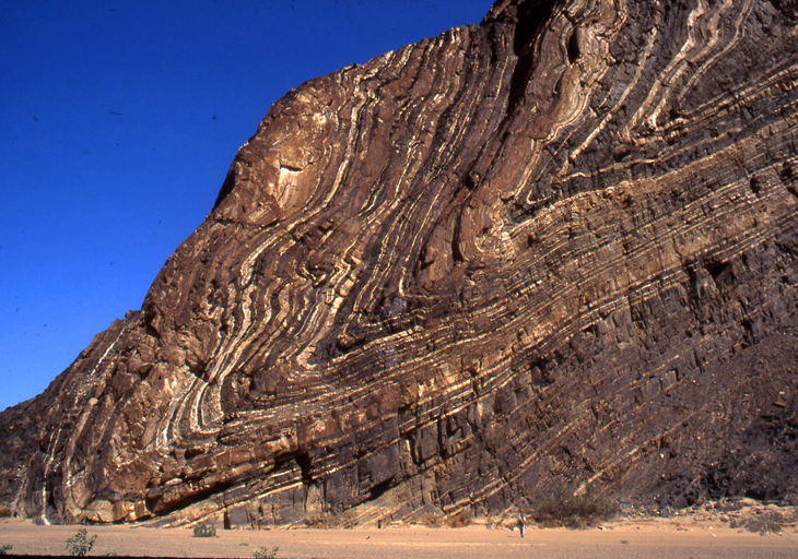
Here are a few images highlighting fold and thrust belts around the world:
 Folded sedimentary layers are a signature of compressional forces associated with mountain-building.


Did I get it?
Plate interiors
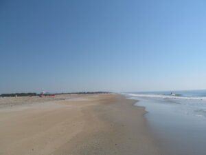
Photo by Doug Kerr via Wikimedia.
.jpg)
Though most of the geological “action” happens at plate boundaries (edges), the vast interiors of plates merit some attention, too. Largely they move as a coherent block, translating in a common direction or rotating around some axis of motion. Passive margins are the “trailing” edges of continents within a plate. For instance, consider the North American continent as it is today. As it moves from east toward the west, the western edge is the active margin (with Cascadia subduction and two giant transform fault zones), and the eastern edge is the passive margin, trailing along with no active tectonics. A place like Virginia is the edge of the continent, but the middle of the plate. No mountains are being actively built in modern Virginia, but old mountains are being eroded away. Particles of sand and mud with origins in the Appalachian Mountains are tumbled downstream and deposited along the western edge of the the Atlantic Ocean.
A passive margin is a site of tectonic calm. Without plate tectonics to rough up the landscape, the topographic relief is minimal. Cool crust is denser, and subsides. This allows the accumulation of deposits of mature sedimentary strata. These sediments (quartz sand, mud, shelly carbonate material) have been laid down along the modern mid-Atlantic margin in the thick layers of the Coastal Plain and continental shelf.
Other modern examples of passive margins include eastern South America, Western Africa, Western Australia, and southern India.
Did I get it?
Variations and mashups
While it is easiest to conceptualize plate boundary types with a neat triumvirate of possibilities, (1) transform, (2) divergent, and (3) convergent, the real world is frequently more complex. Some plate boundary settings “mix” elements of convergent and transform motion. Others mix divergent and transform motion. These situations arise when the direction of plate motion is neither perpendicular nor parallel to the orientation of the plate boundary. Instead, the motion is oblique to the boundary.
Transpression
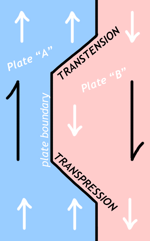
Drawing by Callan Bentley
Transpression is oblique convergence. Two plates converge with one another, but the boundary is oblique to the convergence direction. Rocks caught in a zone of compression are squished and sheared.
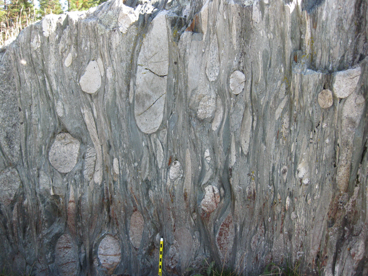
If this occurs at sufficient depth for dynamic metamorphism, they can develop an internal S-C fabric. S-C fabrics are characterized by a wavy, lenticular “grain” to the rock. The waviness comes from the intersection of two planar fabrics: the foliation (“S”) that is typical of so many metamorphic rocks, plus small shear bands (“C”) that cut across and merge with the foliation. Conveniently, the S fabric tends to be wavy, much like the letter S. The C surfaces tend to be more planar, cutting across the S surfaces.
As an example of transpression that might be relevant to a geologist deciphering the tectonic history of a region, consider the GIGAmacro image below. It shows a slab of deformed granodiorite from a Mesozoic-aged transpressional shear zone in the Sierra Nevada of California. Examine the orientation of the light and dark minerals. You can see a diagonal foliation (the “S” surface) as well as a left-to-right series of small shear bands (the “C” surface). This particular pattern indicates that the rock was being compressed “top to bottom” as well as being sheared right-laterally (top to the right):
Cross-sectional view of S-C fabric in Rush Creek Granodiorite, near Gem Lake, California.
GIGAmacro by Robin Rohrback.
S-C fabrics are the deep record of transpression, and are thus reasonably likely to be preserved in the geological record over the long term. Eventually (through uplift, erosion, and exhumation), historical geologists can find S-C fabrics in transpressionally sheared rocks, and extract from them information about which way the plates were moving when those rocks were deformed.
Closer to the surface, transpression may cause the extrusion of soil and rock material vertically. Rock moves upward through ductile flow at depth, but through brittle offsets at shallower depths. This net upward movement of Earth materials makes topographically “high” features, called pressure ridges. We mentioned them briefly above in the context of transform faults where the fault’s orientation is oblique to the relative motion along the fault.
Landscape features are useful to the historical geologist for understanding recent tectonic activity, but the shape of the land is ephemeral, and unlikely to be preserved as useful information over the geological long-term.
Transtension
Transtension is oblique divergence. Two plates diverge from one another, but the boundary is oblique to the divergence direction. Unlike transpression, transtension tends not to last very long as a discrete entity unto itself. Instead, it will rapidly organize itself into a typical “zigzag” pattern of divergent rift valleys and transform faults, as we see along the global oceanic ridge system. For instance, a recent example can be found on the seafloor of the Gulf of California (a.k.a. the “Sea of Cortez”). These, we can see a distinct stairstep pattern to the bathymetry. The Baja California peninsula has been recently ripped off the coast of mainland Mexico and transported to the northwest along a zone of transtension. This transtension has been accommodated through the development of a series of very short segments of oceanic ridge (spreading centers), interspersed along relatively long stretches of transform faults. The transform faults are oriented precisely perpendicular to the ridge axes:
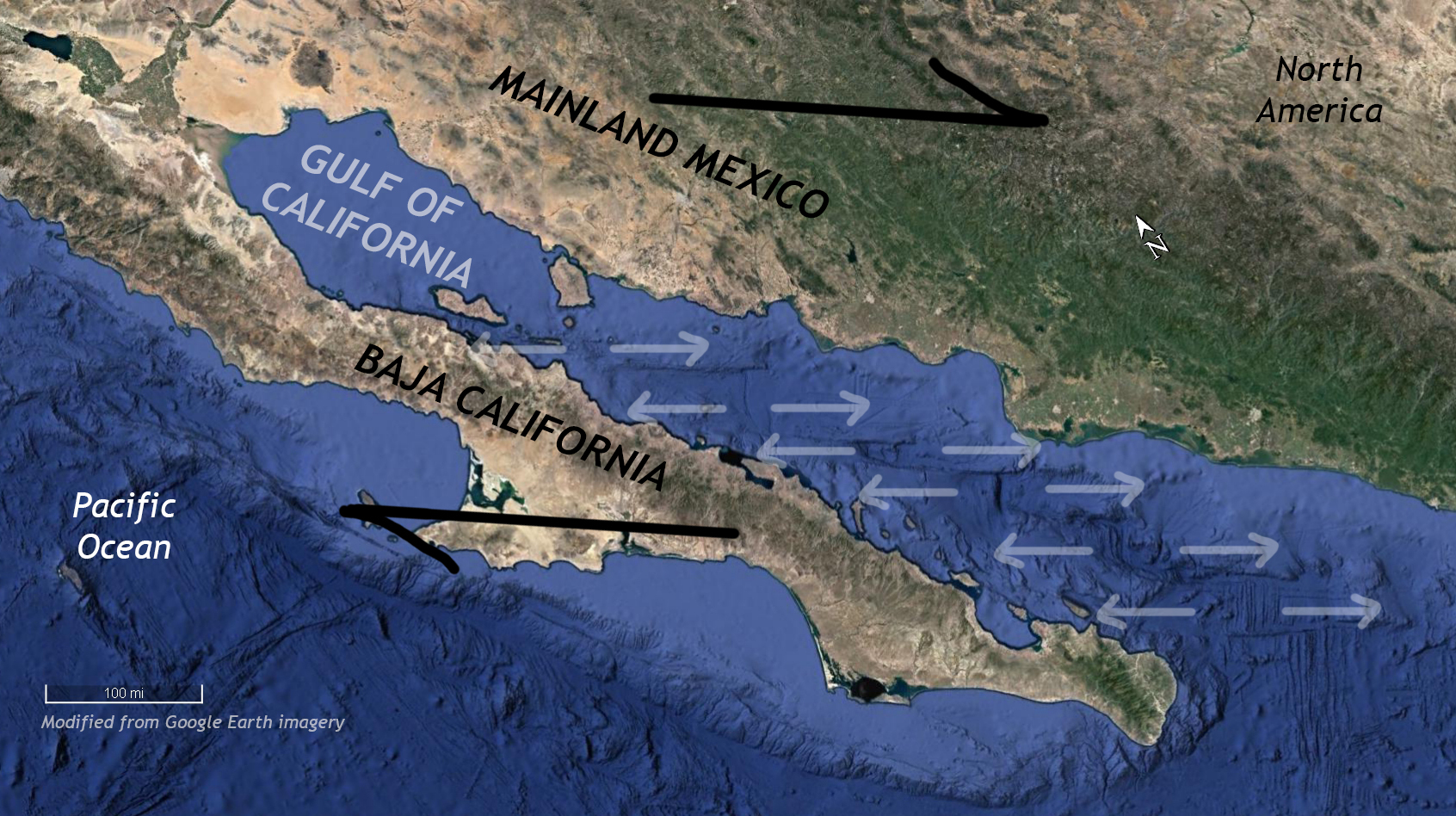
Modified from a Google Earth image.
Example: along the Hayward Fault
Let us now summarize the manifestations of transpression and transtension with a short video looking at the small-scale landforms in Fremont, California’s Central Park, along the trace of the (transform) Hayward Fault:
Did I get it?
The historical record of plate interactions
When plates interact in different ways (convergent, divergent, etc.), various phenomena result. Some of these phenomena are short-lived and thus unlikely to end up preserved in the “deep time” geologic record (offset streams at transform boundaries, for instance). Others create more durable signatures that can be identified in rock millions and billions of years later (such as metamorphic belts of a consistent age, or sedimentary basins that record rifting). When a region experiences divergent tectonics, it forms one set of geological signatures, while a completely different set of rocks, structures, and topography forms as a result of subduction tectonics.
Mountain belts
Convergent plate boundaries between blocks of continental lithosphere are recorded in the geologic record through the construction of mountain belts. When fresh, these mountain belts are mountainous: that is, they show high relief landscapes that occur in linear belts, like the modern Alps or Himalayas. However, intense topographic relief is unlikely to persist in the geologic record. Over time, mountains are worn down by erosion: between landslides, glaciers, and rivers, once-lofty rock is taken downhill, reducing the overall topographic relief.

Cartoon by Callan Bentley.
However, the signatures of mountain-building at the roots of those same mountains may be preserved. These include (1) folded and thrust-faulted sedimentary strata on the flanks of the mountain-belt and (2) foliated metamorphic rocks in the core of the mountain belt. If orogenic temperatures were high enough, some of the minerals in some of the metamorphic rock may melt, forming migmatite. Sufficient partial melting will generate (3) bodies of felsic magma that can cool to form granite plutons. These durable geologic signatures show us where the mountains used to be, even after the mountains themselves are gone.
Callan Bentley photo.
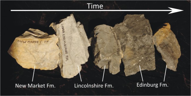
Additionally, consider the situation from the perspective of the stuff that’s removed: the sediment generated by the erosion of the mountains has to go someplace. It goes downhill, and ends up deposited somewhere else, perhaps nearby or perhaps far away, but it adds clastic sediment to the geologic record somewhere adjacent to the mountain belt. A shift in the sedimentary character of a given stratigraphic column from carbonate to clastic can signal an orogeny turning on. Because these clastic strata can contain fossils, we can use their age to determine the timing of mountain-building. A subsequent reversion to carbonate sedimentation thereafter will be a signal that the mountains have been removed as a source of sediment.
Marine sediment shed off a neighboring mountain belt is collectively dubbed flysch. It consists of black shale, bentonite, graywacke, and conglomerate. Terrestrial sediment shed off a neighboring mountain belt is collectively dubbed molasse. Typically it consists of red shale, submature river sandstones, and conglomerate. Before early geologists had come to terms with the non-intuitive ways that metamorphic and plutonic rocks formed, these clastic strata were the first recognized signals of ancient mountain building. The key recognition here is that the bajillions of particles that make up clastic strata represent a tremendous amount of eroded source rock, a huge volume equivalent to vanished mountain ranges.
Cratons and the accretionary growth of continents

Animation derived from Whitmeyer & Karlstrom (2007).
Over time, collisional events between masses of continental crust cause small blobs of crust to glom together and create larger, composite blobs of crust. This map shows the age of the various blocks of crust that make up the North American continent. If the crustal components are old, we tend to call them “cratons,” but if they are more recently tacked on, the preferred term is “terrane.” Whatever the name, the pattern is plain: the oldest bits of crust are surrounded by younger bits of crust. Continents start off relatively small, as resistant blobs of low-density material that survive subsequent collisions with neighboring blobs. Through convergence, they are sutured together and stay together. Seafloor sediment, volcanic island arcs, and other small masses of continental crust merge and stick: continents grow through the accretion of new terranes on their margins.
Ophiolites
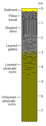
Wikimedia image.
Earlier, we described the structure of the oceanic lithosphere as it forms through seafloor spreading at a divergent boundary. From bottom to top, it consists of mantle peridotite, gabbro, sheeted dikes of basalt, pillow basalt, and that may be topped with deep sea sediments, such as chert or shale. This sequence is both the structure of the oceanic crust as well as the structure of small slivers of rock we often find between accreted terranes. In other words, on dry land, in the heart of mountain belts, we often find what appear to be scraps of oceanic crust. These are called ophiolites. Before the advent of plate tectonics, it was difficult to explain ophiolites, but now we can recognize them as remnant shreds of the oceanic lithosphere that used to separate the two terranes – the scant remains of an ocean basin that was otherwise mostly destroyed through the process of subduction.
For instance, at Gros Morne National Park in Newfoundland, Canada, there is a huge area of exposed peridotite. Though the fresh peridotite would be green because of its olivine content, the wet climate of Newfoundland has rusted it all at Earth’s surface, making the landscape surface orange. Adjacent to the peridotite is layered gabbro, and adjacent to that are sheeted dikes and pillow basalts.
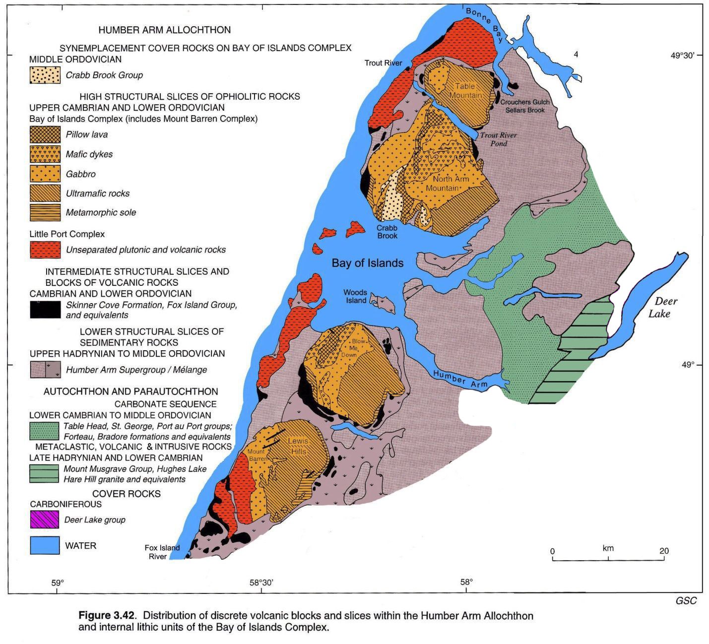
Geological Survey of Canada map.
The record of subduction
Callan Bentley photo.
Subduction is a key component of plate tectonics. To recognize places where subduction has occurred in the geologic past, we look for metamorphic, igneous, and structural signatures. One of the basic aspects of modern subduction is the parallelism of oceanic trench and volcanic arc. These two settings have different blends of temperature and pressure, resulting in different “flavors” of metamorphic rocks. The trench and Wadati-Benioff zone will result in high pressure + low temperature metamorphic rocks, while the neighboring magmatic arc will produce moderate pressure + high temperature metamorphic rocks. These “paired metamorphic belts” allow us to distinguish the earliest records of subduction from the geologic record, and the rather different tectonic situation that preceded subduction during the Archean.
Few places preserve this better than coastal northern California. The rock there formed (and deformed) during the Mesozoic subduction of the Farallon Plate beneath the western North American Plate.
Did I get it?
Sedimentary basins
An important consequence of plate tectonics for Historical Geology is how the different plate boundary settings give rise to circumstances where sediments can accumulate and be preserved over the geological long term. Substantial loci of sedimentary deposition are referred to as basins.
Transform
Because transform plate boundaries largely conserve the land surface as it is, merely offsetting it in opposite directions, they do not tend to be exceptionally good basin formers. However, where there are small “jogs” in the orientation of the fault trace, transtension can open up relatively small wrench basins.
Wrench basins

Modified from Google Earth imagery.
Wrench basins form when a right-lateral fault steps over to the right, or a left-lateral fault steps over to the left. The land between the end of one fault segment and the beginning of the next will sag. As we saw above, on a small scale this can generate a sag pond (or a low spot in a parking lot!), but on a larger scale it can produce substantial basins: these catchments dilate and create a topographic low spot into which sediment can pour from the surrounding highlands.
The Dead Sea, on the boundary between Israel, the West Bank, and Jordan, is an excellent modern example. Here, the Dead Sea Transform Fault, a left-lateral series of faults between the Sinai Peninsula and the Arabia Plate. As at Aqaba, and the Sea of Galilee, left steps in the fault system have stretched open low spots in the landscape, filled by water. At Aqaba, it’s an offshoot of the Red Sea. The Sea of Galilee is landlocked, and filled with freshwater.
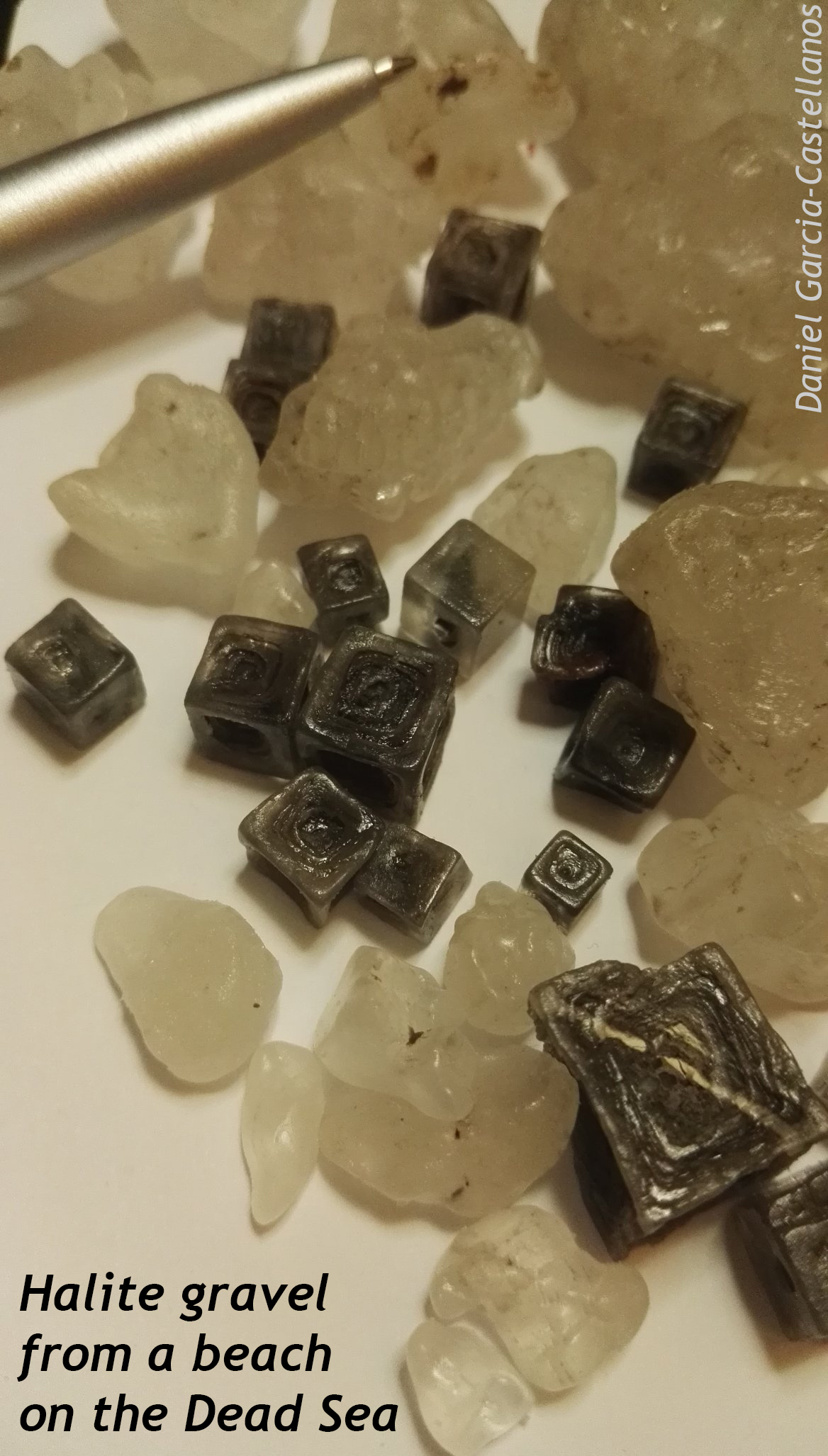
Photo by Daniel Garcia-Castellanos; reproduced with permission.
The Dead Sea is the lowest spot on land in the entire world. (There are of course, deeper spots in the ocean basins, such as the Marianas Trench.) The hot, dry climate and lack of replenishing water (especially in recent years) have resulted in an extremely salty body of water occupying the basin, currently at 430.5 meters below sea level (-1,412 feet in elevation), but dropping further every year.
Other modern examples include the Salton Sea (on the San Andreas Fault) and the Sea of Marmara (south of İstanbul on the North Anatolian Fault).
Wrench basins are not just a modern phenomenon, however. In true uniformitarian spirit, we find many preserved in numerous contexts in the geologic record. They can serve as excellent repositories of local lithologic diversity in situations where the source rocks have been completely eroded away.
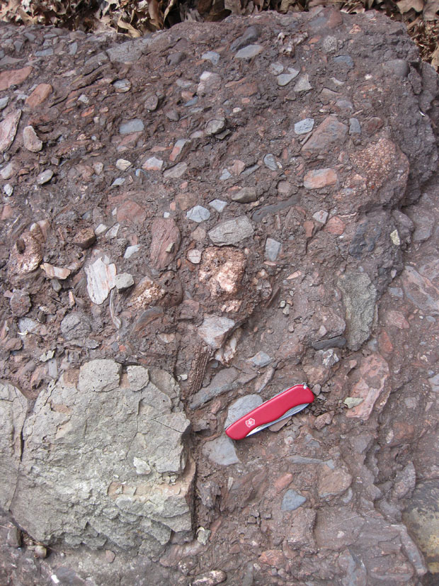
Callan Bentley photo.
For instance, in the heart of the Superior Craton of North American, there are a series of wrench basins that captured cobbles derived from the surrounding highlands: mountains that haven’t seen topographic relief since Archean times. Thanks to the preservation of these wrench basin conglomerates, we can see not only which areas were made low by tectonics, but what composition rocks made up the surrounding high country.
Divergent
Callan Bentley photo.
The principal variety of basin that forms at a divergent setting is a rift basin. When rift basins are fresh, they accumulate immature clastic sediment. Over time, especially in large rift basins, the sediments may mature towards a higher proportion of quartz and clay. Some even see limestones at positions far removed from the basin margins. Volcanism is important too: as the crust stretches in a rift, it lowers the pressure on the underlying mantle. Decompression melting follows, which produces mafic magma. Eruption of basalt and intrusion of gabbro and diabase are common igneous features of rift basins.
Rift basins
As we’ve already mentioned, the Great Rift Valley system of east Africa offers an outstanding modern example of a rift basin. Because of its location and timing, this is *the* place to look for fossils of human ancestors. Other modern examples of rift basins include Lake Baikal in Siberia (and a smaller equivalent to the south in Mongolia, Lake Khovsgol). The valley of Þingvellir (“Thingvellir”) in southwest Iceland, is celebrated by Icelanders as the seat of the world’s oldest functioning democracy, but geologists see it in a different light: it is a place where the Mid-Atlantic Ridge can be seen above sea level. All of these basins are bound by normal faults.
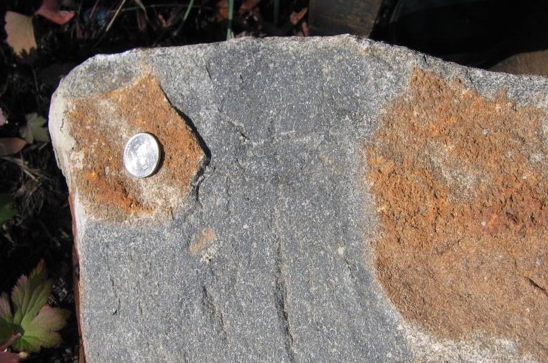
A fine example of an ancient rift basin can be found in central Virginia, where the Culpeper Basin is the largest of a dozen basins that preserve terrestrial sediments (and mafic igneous rocks) related to the break-up of the supercontinent Pangaea and the initial opening of the Atlantic Ocean.
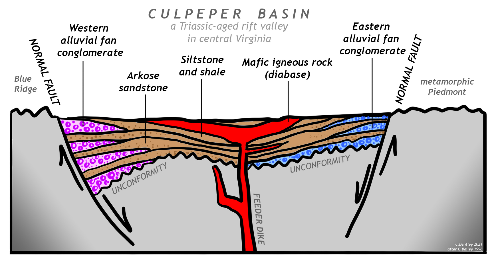
Callan Bentley cartoon.
The Culpeper Basin is filled with clastic sediment and mafic igneous rock. It shows coarsest-grained sediment at the margin basins. These alluvial fan deposits are different in composition in the west versus the east, as the alluvial fans in the two locations were draining highlands of very different compositions. In the west, limestone and basalt clasts predominate. (One of these western fanglomerates, the Leesburg Conglomerate, makes up the distinctive columns of the Hall of Statuary in the United States Capitol building.) In the east, the large clasts are mainly foliated metamorphic rocks derived from the neighboring Piedmont geologic province. Further from the basin margins, the sediments get finer. They include arkosic sands and mud deposits.
.jpg)
Lake deposits from the central Culpeper Basin have been contact metamorphosed to yield layers of multicolored hornfels that produce surprisingly durable cliffs:
Contact-metamorphosed meta-mudstones (rift valley lake sediments) of the Triassic Balls Bluff Formation exposed in road cuts along the Dulles Greenway between Reston and Leesburg, Virginia.
GigaPan by Chris Johnson.
The Culpeper Basin is one of many basins that formed in the heart of Pangaea during its breakup. Some of these basins connected up — a line of “weakest links” — and ripped open to make the Atlantic Ocean. Basins east of that line are now in Africa and Europe. Basins west of that line, including the Culpeper Basin, are called the “Newark Supergroup” basins. Other examples in this collection include the Gettysburg Basin, the eponymous Newark Basin, the Hartford Basin of Connecticut, and Canada’s Bay of Fundy. Collectively, the Newark Supergroup basins are quite extensive.

Callan Bentley photo.
Another huge rift basin can be found in northwestern Montana and adjacent states and territories: the Belt Supergroup was deposited in the Belt Basin in Mesoproterozoic sedimentary time. Like the Culpeper Basin, it’s coarsest at the edges and at the bottom. It’s also similar in having intercalated mafic igneous rocks. It’s different in being much larger, and lasting long enough to develop more mature sediments, including thick carbonate packages within its stratigraphic sequence.
Modified from a USGS map; explore more here.
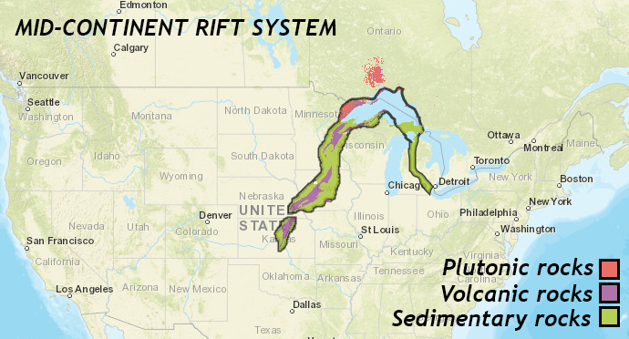
Another ancient rift basin worth noting is the Mid-Continent Rift of North America (also called the Keweenawan), which extends from Lake Superior in Minnesota to the southwest, diving beneath sedimentary cover for much its length (but still detectable via its distinctive positive gravity anomaly signature). This gigantic rift system developed in the Mesoproterozoic immediately before the Grenville Orogeny.
Convergent
Subduction at convergent plate boundaries can also induce sedimentary basins to form. There are three principal varieties to consider: foreland basins, forearc basins, and backarc basins.
Foreland basins
Foreland basins form on the continental crust as subduction loads the crust with a heavy mountain range. Thrust faulting thickens the crust adjacent to a subduction zone, and this additional rock mass causes the adjacent crust to sag. The sagging creates accommodation space for sediment.
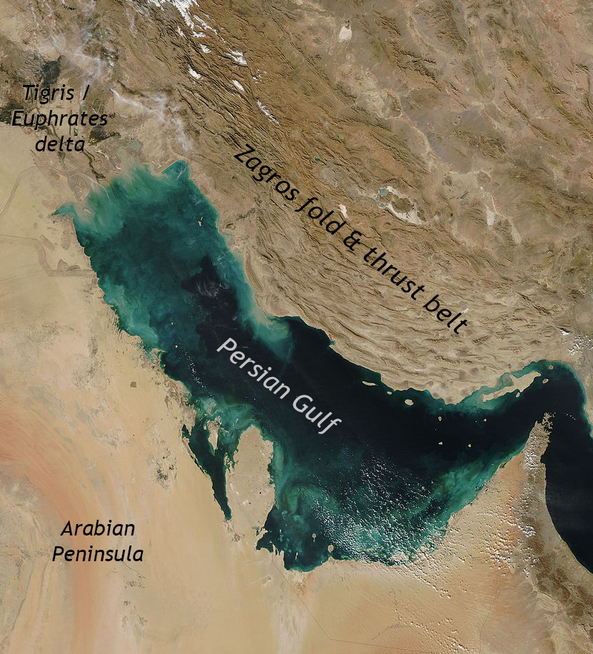
A modern foreland basin can be seen in the Persian Gulf. The Persian Gulf is a foreland basin between the Arabian Peninsula and the southern edge of Eurasia: Iran’s Zagros Mountains. As the Arabian Plate and the Eurasian Plate converge, thrust-loading of the crust in the Zagros has caused the adjacent crust to sag and make the low spot of the Persian Gulf.
An Ordovician example can be found in the mid-Atlantic region: the Queenston clastic wedge is a thick package of sediment including both marine flysch and terrestrial molasse that formed in response to downward flexure of the crust induced by the Taconian Orogeny. The same pattern repeated during the Devonian Acadian Orogeny [LINK NEEDED]: the Catskill clastic wedge is the name given to this subsequent foreland basin, partially overlapping in space the region occupied by its Ordovician predecessor.
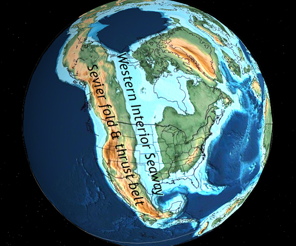
Modified from a paleogeographic map by Christopher Scotese.
In Cretaceous western North America, another foreland basin formed: the Western Interior Seaway stretched from the Gulf of Mexico to the Arctic Ocean. Seawater flooded a vast trough of land that sagged downward as subduction of the Farallon Plate caused the Sevier Orogeny. This episode of thin-skinned deformation thrust thick slices of sedimentary rock into towering peaks.
Forearc basins
Forearc basins form on the trench side of volcanic arcs. Subduction at the trench keeps the crust low, and the neighboring volcanic arc sheds copious sediment that can fill the basin.

Photo by Diliff, via Wikimedia Commons.
A classic example is the Great Central Valley of California, which is a forearc basin of Jurassic/Cretaceous age. At that time, subduction of the Farallon Plate generated a thick accretionary wedge of seafloor rocks. This is preserved in the modern day as the bulk of California’s Coast Ranges. Inland, this same subduction manifested as a vibrant volcanic arc, the roots of which are today preserved as the Sierra Nevada batholith, the voluminous wad of granites that can be found in places such as Yosemite National Park. During the Cretaceous, the Sierra Nevada would have looked much like the modern Andes Mountains of South America. Though the volcanoes themselves have since been eroded away, the extent of their source magma chambers is gloriously revealed in the high country of that excellent mountain range.
Between the Coast Ranges’ accretionary wedge and the Sierra’s magmatic arc is the vast, hyperflat Great Central Valley. Though the valley is a modern topographic low, it corresponds very closely in areal extent with the Cretaceous submarine forearc basin:
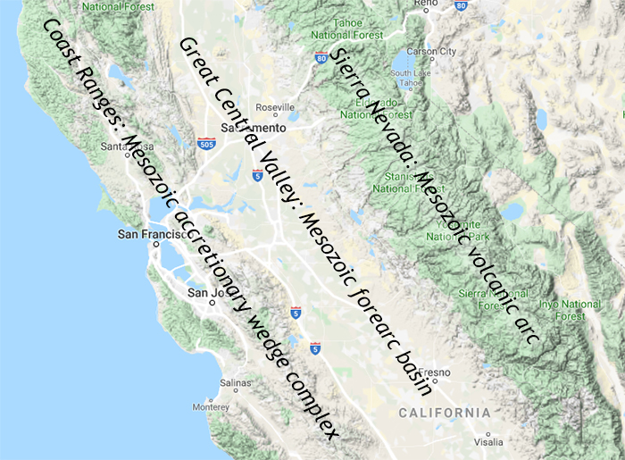
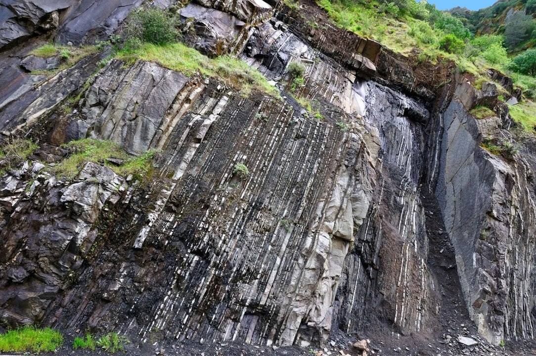
Photo by Mike S. Clark via Wikimedia.
The Great Central Valley is 60 to 100 km (40 to 60 miles) wide. It stretches approximately 720 km (450 miles) along a north-northwest to south-southeast trend, paralleling the volcanic arc to the east and the accretionary wedge to the west. Clastic sediments deposited in this basin make up the 12 km-thick (40,00o’) Great Valley Sequence. Mostly shale, it also includes substantial bodies of sandstone and conglomerate that probably represent Mesozoic abyssal fan systems, sourced from the Sierra Nevada volcanic arc.
Back-arc basins
Callan Bentley cartoon.
Back-arc basins are the final category associated with convergent boundaries. There’s a plot twist though: ironically, they actually require divergence to form! They result from tensional forces caused by rising mantle material coupled with oceanic trench rollback (the oceanic trench shifts over time in the direction of the source of the subducting plate). The arc crust is under extension or rifting as a result of the sinking of the subducting slab. A good modern example of back-arc spreading is the Sea of Japan, a modest ocean basin that has opened between the islands of Japan (a volcanic arc) and the Asian mainland.
Did I get it?
Geophysical phenomena
Several manifestations of plate tectonics are best examined through the lens of geophysics.
Earthquakes
The vast, vast majority of earthquakes on Earth are associated with plate boundaries. Examine this map showing more than a century of epicenters to get an immediate, visceral sense of this pattern:
Earthquakes are caused by the sudden slip of two bodies of rock past one another, after tectonic stresses have accumulated to the point that they overwhelm frictional inertia. Most (95%) of the places where rock is forced into the uncomfortable position of scraping over other rock are located at plate boundaries. The exceptions (5%) are at sites where the crust is being stressed for other reasons: excessive loading due to sedimentation, intrusion of magma, isostatic adjustments, or artificially induced seismicity due to elevated pore pressure.
Volcanoes
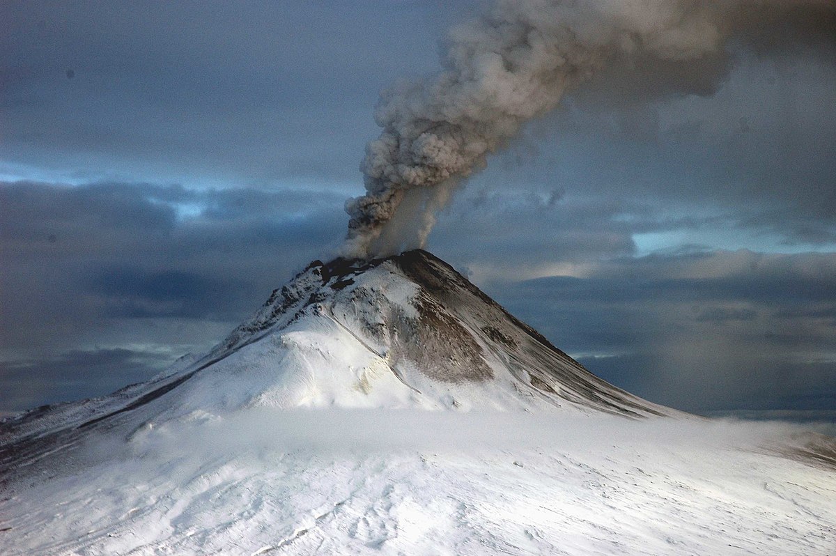
Photo by Game McGimsey, USGS.
Similarly, most volcanoes on this planet are associated in some way with plate boundaries [map]. There are four major options here:
-
- Subduction of oceanic lithosphere under continental lithosphere (example: Andes)
- Subduction of oceanic lithosphere under oceanic lithosphere (example: the Philippines)
- Divergence (rifting) of continental lithosphere (example: East African Rift)
- Divergence (seafloor spreading) of oceanic lithosphere (example: Mid-Atlantic Ridge)
But volcanoes can also form in non-plate boundary settings. When we find eruptions piercing plates in locations far from their edges, many geologists invoke hot spots or mantle plumes. The idea here is that, independent of plate motions, the mantle has isolated point loci where rising warm material convects upward, and in so doing partially melts. The magma makes its way through the overlying lithosphere and erupts. This can occur in a couple of contexts:
-
- Hot spot volcanism through oceanic lithosphere (example: Hawaii)
- Hot spot volcanism through continental lithosphere (example: Yellowstone)
GPS & InSAR
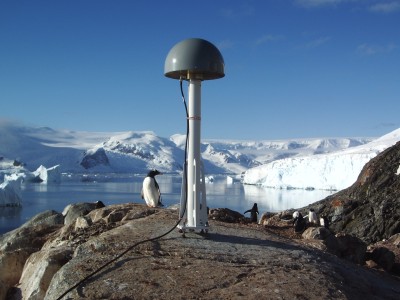
UNAVCO photo.
One of the greatest innovations of the modern era is the advent of global navigation satellite systems (GNSS), including the American global positioning system (GPS). With dozens of satellites orbiting the Earth, a given receiver on the ground can trilaterate its position exceptionally precisely. This is not only useful for Waze getting you to your job interview on time, but can also be used for documenting the subtle motions of Earth’s crust.
GNSS measurements show the crust moving relative to other parts of the crust. To analyze GNSS information, a geodesist must choose a frame of reference. Since no spot on Earth’s surface is stationary over the long term, it is important to realize that all plate motion is relative to other plates. For instance, if you choose North America as your reference frame, but examine the motions of various spots west of the Wasatch Front, you’ll find an interesting set of patterns:
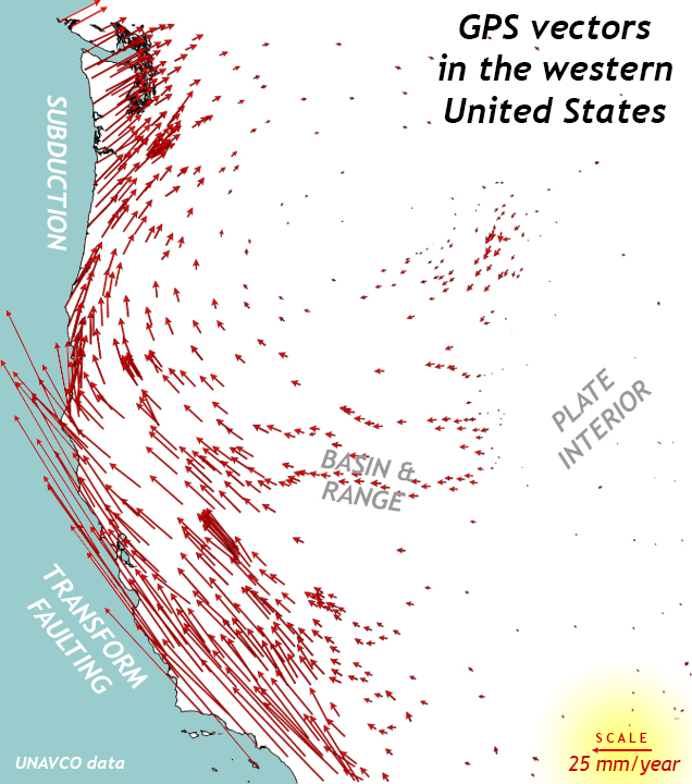
UNAVCO data.
Each arrow shows the vector of motion* of that location. Vectors are ways of describing motion in terms of both magnitude and direction. The longer the arrow, the faster that bit of the crust is moving. The arrow points in the direction that crust is moving relative to the North American frame of reference.
*Technically, what is shown in that map is the horizontal component of the velocity. There can also be a vertical component of the velocity (i.e., up or down motion), especially at divergent or convergent boundaries, or sites of transpression or transtension. Displaying this vertical motion is an additional option on the UNAVCO GPS Velocity Viewer application.
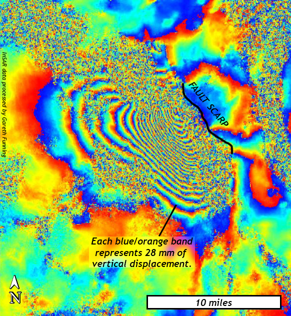
Modified from an original interferogram by Gareth Funning.
Another aspect of satellite measurement can be utilized for examining land positions before and after an earthquake. InSAR uses microwaves to repeatedly measure the shape of Earth’s surface, and if there is a change (sudden or gradual), InSAR can detect the difference between one radar mapping “pass” by a satellite and its successor. What’s literally being measured here is whether the land surface has moved toward or away from the satellite. InSAR data is displayed in rainbow-scale maps called “interferograms.” Each psychedelic blue/orange band in such an image represents a vertical displacement of 28 mm. Counting the number of bands and multiplying by 28 will give a fair estimate for the vertical offset of a fault in a given earthquake, as measured in millimeters.
Did I get it?
Driving forces
The magnitude and direction of lithospheric plate movement is the result of the various forces acting on the plate, and the plate’s resistance to those same forces. What could make such a massive slab of rock overcome inertia and move though geologic time? Convection in Earth’s mantle is relevant, but probably greater momentum comes from the forces of ridge push and slab pull.
IRIS video.
Callan Bentley photo.
When oceanic lithosphere subducts to a sufficient depth, the basalt is metamorphosed to blueschist and then eclogite. Eclogite is particularly dense (3.45 to 3.75 g/cm3), and that extra dense material on the leading edge of the subducting slab may yank on the rest of the plate with an urgency that cannot be resisted. In other words, the metamorphic reactions that make eclogite help contribute to the slab pull force.
Did I get it?
Wilson Cycles
It is critical for historical geologists to recognize that the dynamics of a given plate boundary (divergent, convergent, etc.) are not eternal. A given spot on Earth’s surface may be divergent for some time, then convergent, then divergent again. Just because a given place is tectonically inactive today, that doesn’t mean it was not active in the past. Things change!
From the perspective of continents, another way of putting this is to say: supercontinents form, and then break up. A given spot on a continent may be a site of divergence and rifting (opening up a new ocean basin next door), and later a site of convergence and mountain-building (as that ocean basin is closed and the continents on either side collide). Tuzo Wilson recognized these signatures and described them in a classic 1966 paper about the opening and closing of ocean basins. Because he was first to publish the idea that the change of tectonic setting could be cyclical, we often refer to supercontinent cycles as “Wilson cycles” today.
Mid-Atlantic Wilson Cycles
The eastern margin of the United States offers a classic example of how a given place can shift from convergent to divergent to passive to convergent to divergent to passive again. These sequential shifts accompanied the construction of two subsequent supercontinents (Rodinia and Pangaea) and their subsequent break-up. These repetitive “cycles” of supercontinent formation and destruction are particularly well recorded in the Appalachian mountain belt.
At locations up and down the east coast of North America, there are four major batches of active tectonism, interspersed with times of passive margin conditions:
-
-
- From 1.2 to 1.0 Ga, mountain-building dominated, marked by granites, metamorphism, and deformation. This made the supercontinent Rodinia.
- From 700 Ma to 565 Ma, rifting dominated, marked by mafic volcanism and immature sedimentary deposits. This broke Rodinia up into fragments, and opened the Iapetus Ocean between them.
- Subsidence and passive margin sedimentation occurred through the Cambrian and early Ordovician (~550 to ~480 Ma).
- From 300 to 250 Ma, mountain-building dominated, marked by granites, metamorphism, and deformation. This made the supercontinent Pangaea.
- From 200 to 180 Ma, rifting dominated, marked by mafic volcanism and immature sedimentary deposits. This broke Pangaea up into fragments, and opened the Atlantic Ocean between them.
- Passive margin sedimentation resumed, from the Cretaceous (~100 Ma) until today.
-
The Grenville Orogeny

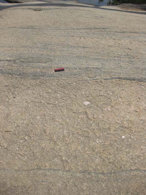
Callan Bentley photo.
The oldest rock on the east coast of North America is intrusive. Much of it is felsic in composition, reflecting the partial melting of older source rocks. Dating zircons from these granites and granite gneisses of the “basement complex” gives ages of 1.2 to 1.0 Ga. In general, the older units are more foliated than the younger units, suggesting they were around for a longer period of time during mountain building, with more time to build up a pervasive compressional fabric. Basement rocks of this age are found from Texas to Newfoundland, including the anorthosites making up the Adirondack Mountains in New York, and the granites of the Blue Ridge province in North Carolina and Virginia.
Iapetan rifting
Callan Bentley photo.
When Rodinia broke up, it was marked by the intrusion of mafic dikes and the eruption of large volumes of mafic lava. The resulting flood basalts bear vesicles, xenoliths, and cooling columns. Normal faulting led to rift valleys that filled with immature clastic sediment, including gravel, arkosic sand, and mud. Some of these rift basins connected up, becoming “the weakest link” between ancestral North America (Laurentia) and the various Proterozoic continental fragments that drifted away from it. Seafloor spreading took over, filling in the gap between continents with fresh injections of basalt. The Iapetus Ocean was born. Inch by inch, this ocean basin widened for hundreds of millions of years, adding a “skirt” of oceanic crust to the edge of the ancestral North American plate.
Appalachian mountain-building
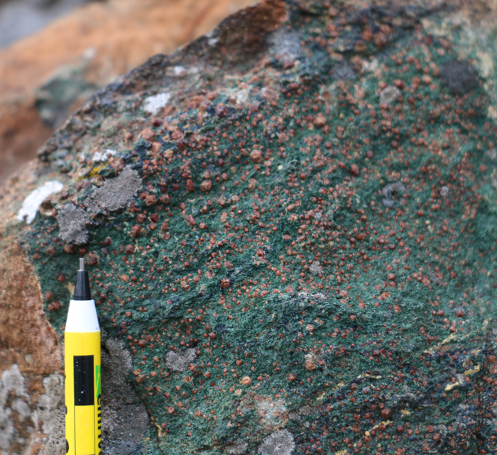
Callan Bentley photo.
The Appalachian Mountains mark the suture between ancestral North America (Laurentia) and ancestral Africa (the leading edge of Gondwana). They represent the collision between these two large continental landmasses, formerly separated by the Iapetus Ocean. Over the course of the Paleozoic, the Iapetus began to close (resulting in two earlier, smaller orogenies), and the temporary “skirt” of oceanic crust was recycled into the mantle via subduction. This brought Africa and North America ever closer, until eventually they merged in a collisional mountain belt. When the Appalachians were young, they ran through the heart of the Pangaean supercontinent on a scale that may have dwarfed the modern Himalayas. Based on the age of the rocks deformed by compressional stresses and the dating of granites and metamorphic rocks, it appears that the final orogeny occurred in the late Paleozoic, starting around 300 Ma (in the Pennsylvanian) and wrapping up by about 250 Ma (in the Permian). This compressional event resulted in the folding and faulting of older strata in what is today the Valley & Ridge province, metamorphism of the rock in the Blue Ridge and Piedmont province, intrusion of granite plutons, and suturing of African crust to the North American crust.
Atlantic rifting
Callan Bentley photo.
When Pangaea began to break up in the Triassic, the tectonic extension was first marked by the intrusion of mafic dikes. Normal faulting resulted in the opening of numerous parallel rift basins up and down the east coast. Some of these rift basins connected up, becoming “the weakest link” between North America and Africa/Europe. They stretched wide enough apart that seafloor spreading took over, filling in the gap between continental fragments with fresh injections of basalt. Inch by inch, the Atlantic basin has been widening ever since. Numerous “failed” rift basins remain in the Piedmont geologic province, sort of like “stretch marks” in the crust. They are dominated by two kinds of rocks: immature clastic sediments, and mafic volcanics. The immature clastic sediments include conglomerates and arkose sandstone near the margin of the basins, but also lake deposits in the basins’ centers.
Did I get it?
References, citations, and further reading
Kim Blisniuk (2019). “San Andreas Fault at Sanborn County Park,” Streetcar 2 Subduction virtual field experience using Google Earth. American Geophysical Union.
Chris Johnson, Matthew D. Affolter, Paul Inkenbrandt, & Cam Mosher (2017). “Plate tectonics,” An Introduction to Geology, OER textbook: CC-BY.
Erik Klemetti (2020), “Are we seeing a new ocean starting to form in Africa?,” Eos, 101, https://doi.org/10.1029/2020EO143740. Published on 08 May 2020.
Geoff Manaugh (2019), “Move Over, San Andreas: There’s an Ominous New Fault in Town,” WIRED, April 18 2019.
Naomi Oreskes (1999), The Rejection of Continental Drift: Theory and Method in American Earth Science. Oxford University Press: 432 pages.
Matthew E. Pritchard (2006). “InSAR, a tool for measuring Earth’s surface deformation,” Physics Today, July 2006, pg. 68-69
Dale Sawyer (2005), “Discovering Plate Boundaries,” Rice University website (teaching activity).
Tom Simkin, Robert I. Tilling, Peter R. Vogt, Stephen H. Kirby, Paul Kimberly, and David B. Stewart (2006). “This Dynamic Planet,” Cartography and graphic design by Will R. Stettner, with contributions by Antonio Villaseñor, and edited by Katharine S. Schindler. USGS map.
UNAVCO (2021). GPS velocity viewer. Website.
UNAVCO (2019). InSAR: Measuring the changing shape of our Earth from above. Informational poster [back].
Ben van der Pluijm, Christopher Scotese, and Josh Williams (2020). Deconstructing Tectonics. Google Earth tour.
J. Tuzo Wilson (1966), “Did the Atlantic Close and then Re-Open?” Nature 211, 676–681. https://doi.org/10.1038/211676a0
Steve Whitmeyer and Karl Karlstrom (2007). “Tectonic model for the Proterozoic growth of North America,” Geosphere 3, p. 220–259, doi: 10.1130/GES00055.1
_______________________________
A printable PDF copy of this page is here.
Chapter Contents