Plate tectonics is an overarching paradigm that explains a lot of independent observations about Earth surface dynamics. In this case study, we examine the historical development of this important idea. A separate chapter outlines a modern treatment of plate tectonics.
After sputtering suggestions of continental movement in the previous 150 years (most notably in 1915), new information about the seafloor between the continents was revealed in the aftermath of World War II’s naval battles. This prompted a fresh look at crustal dynamics, and in the late 1960s and early 1970s, geoscientific consensus gelled around the idea that many different observations about our planet could be explained with a single model. The idea of “plate tectonics” put together old ideas about continental drift with new data showing seafloor spreading. The new theory was a revolutionary explanation that made the distribution of volcanoes, earthquakes, continents, and topography make sense in a way that no idea had achieved before. Fifty years of additional data and testing have confirmed plate tectonics as the key idea in modern geology.
Antecedents
The idea that continents can move is a rather audacious notion to emerge in the mind of an human who lives such a short life. Prior to the invention of satellite-based telemetry (GPS), there was not discernible way to directly measure such a thing. Yet various lines of evidence did suggest the notion to various thinkers in the European scientific tradition. A particular prompt came from the mapping of the world’s landmasses as a consequence of the “Age of Exploration.” (That’s a Eurocentric phrase if ever there was one! Sometimes this is called the “Age of Being Explored by Europeans,” since that is how most of the world’s population experienced it.) Once the shapes of other continents were documented, they could be contemplated.
The earliest mention of what could later be called continental drift appears to have been Abraham Ortelius. In 1596, he mused on the shapes of the Atlantic coastlines of the Americas, Europe and Africa. Their shapes were so similar, he suggested that they may have been “torn away… by earthquakes and floods.”
Almost 300 years later, in 1858, Antonio Snider-Pellegrini published his hypothesis of continental drift, using the shapes of the continents as his primary line of evidence, but also citing similar terrestrial fossils on widely separated continents. These lines of evidence would also be invoked by Alfred Wegener.
Did I get it?
Continental drift
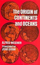
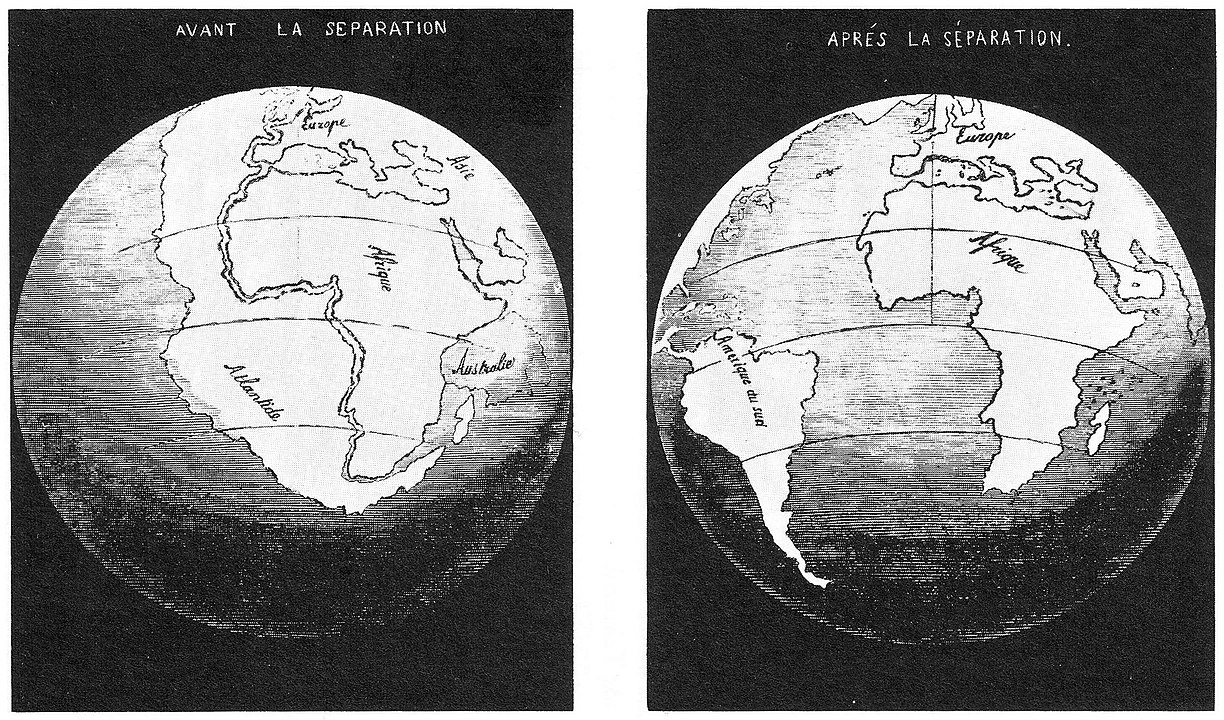
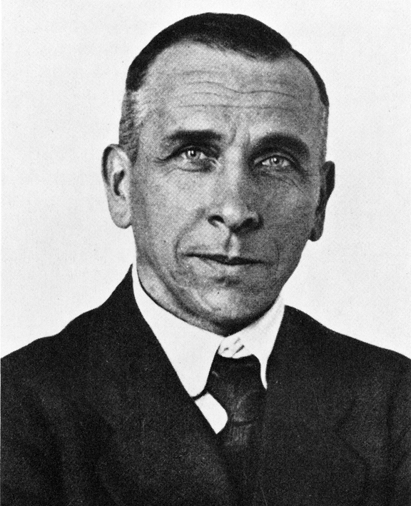
German meteorologist Alfred Wegener compiled evidence for continental movement through time, first sharing these ideas in a 1912 talk and then later publishing a 1915 German book called Die Entstehung der Kontinente und Ozeane (‘The Origin of Continents and Oceans’). In it, he postulated the existence of a supercontinent he called Pangaea which existed in the late Paleozoic Era. According to Wegener, since the early Mesozoic, Pangaea’s various pieces have been drifting away from one another, with the Atlantic Ocean opening up in between. He is the person most associated with a full-throated articulation of the idea of continental drift.
Marshalling evidence for this audacious idea, Wegener compiled evidence of several varieties:
-
- the shape of the continents
- modern mountain belts
- ancient mountain belts
- sedimentary rocks that indicated paleo-latitude
- glacial striations
- the distribution of fossil organisms
Let us examine each in turn.
The shape of the continents
Like Snider-Pellegrini, Wegener first conceived of continental drift by noting the visual match between the shapes of the continents, particularly South America’s eastern coast and Africa’s western coast. The fit between these two is even more pronounced when the modern coastline is ignored, and instead the “puzzle pieces” are defined on the basis of the edge of the continental shelf. Though currently submerged by seawater, the edge of the shelf is where the continental crust truly ends.

Charles Hamm photo, via Wikimedia.
But while his predecessors stopped there, Wegener took the idea further. After all, jigsaw puzzles are solved not only only on the basis of the shape of their pieces, but the imagery on their surface too. So Wegener examined the geological evidence on the continents themselves, comparing these data across the oceans in an attempt to match them up.
Modern mountain belts
One compelling line of evidence for continental drift comes from modern mountain belts.
Once you substract the Atlantic Ocean, the Appalachian Mountains line up with other ranges, including the Caledonides in Scandinavia, the North-west Highlands of Scotland, and the Anti-Atlas Range in Morocco. The mountain belts running through Scotland and Newfoundland fill in some of the connective tissue, and suddenly this appears to be a single mountain range, running through the former heart of Pangaea, now ripped asunder into several pieces.
Here is a reconstruction of Pangaea presented as a paleogeographic map, so you can zoom in and examine the linear trend of the pre-Atlantic mountain belt for yourself:
Paleogeography of the Permian (~250 Ma).
Maps by Christopher Scotese of the PALEOMAP project, with virtual globe by Ian Webster of Dinosaur Pictures.org; reproduced with permission.
Ancient mountain belts
Callan Bentley cartoon.
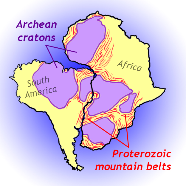
Mountain ranges aren’t stable topographic entities. All that rock poking up into the air represents a lot of potential energy. Landslides and rockfalls tear mountains down over geologic time, reducing their topographic relief. But we can still tell where the mountains used to be on the basis of geological evidence including (1) belts of foliated metamorphic rocks, (2) granite intrusions, (3) zones of compressional deformation — folding and thrust faulting, all at the “roots” of ancient mountain belts, and (4) deposits of sedimentary rock adjacent to the mountain belt (and derived from it). Wegener used the pattern of Proterozoic-aged mountain belts that wrapped around more ancient blocks of continental crust as an additional line of evidence of the former connection of Africa and South America.
Sedimentary rocks that indicate paleolatitude
Callan Bentley graphic using NASA imagery.
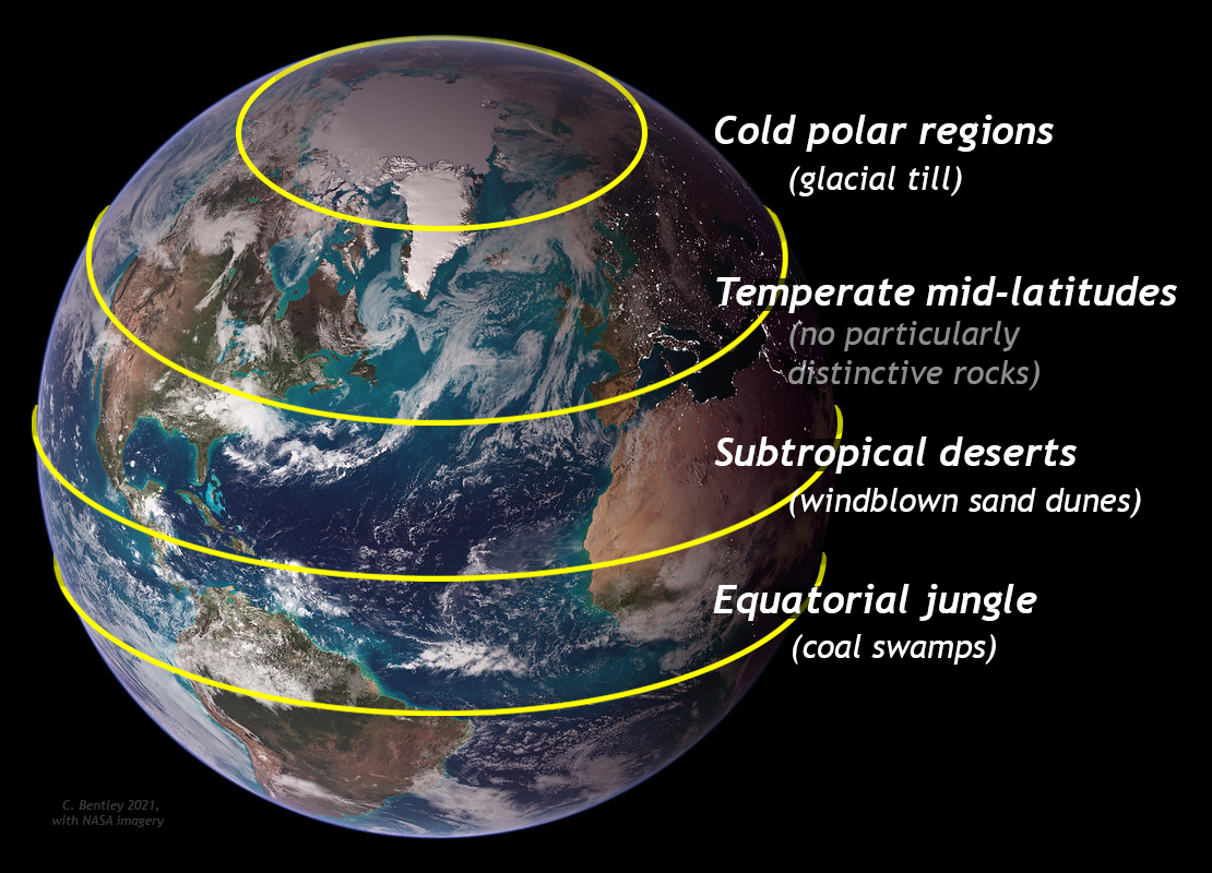
One of the big, obvious patterns about our planet today is that it’s colder toward the poles and warmer toward the equator. Applying the principle of uniformity (a.k.a. “uniformitarianism“) to the ancient past, Wegener reasoned that during the time of Pangaea, the same pattern applied. The idea here is that the positions of landmasses in the past might be indicated by characteristic deposits of sediment on their surfaces. In other words: certain sedimentary rocks form in cold settings only, while others are more likely in the tropics or mid-latitudes. Wegener deduced that Pangaea was a Permian-aged supercontinent, so he looked at the character of Permian-aged sedimentary rocks found on the various continents. South Africa showed diamictites of glacial origin, and therefore was in a polar position at Pangaean times. He also identified a belt of coal, which he interpreted as representing thick forest cover thriving at the Pangaean equator. Flanking the coal belt were two belts of windblown sand, stacked up in dunes that resembled those in the modern Sahara Desert. Wegener interpreted these as representative of the subtropical high-pressure zones where atmospheric circulation nurtures deserts today.
The key thing about all these observations is that they held up across continents, like a series of colored stripes extending across multiple jigsaw puzzle pieces.
Glacial striations

Photo by Evelyn Mervine; reproduced with permission.
We mentioned sedimentary rocks that served as evidence of Permian-aged glaciation in the southern part of Pangaea. There is a tangent worth exploring here, too – or at least Alfred Wegener thought so! When glaciers flow over the landscape, they gouge into it. This can create spectacular U-shaped valleys, but on a smaller scale, the glacier carries a suite of boulders and cobbles and that get scraped over the landscape as the glacier flows. This leaves behind a series of parallel striations. These linear features show which way the glacier flowed. By comparing striation orientations from Permian-aged unconformities in different parts of southern Pangaea, Wegener was able to reconstruct a radial pattern, like the spokes on a bicycle wheel. He interpreted this as the pattern you would expect from a single ice sheet, like modern day Greenland, where a big domelike mass of ice flows downward and outward in all directions. (The Greenland ice sheet was a place he was very familiar with.) The center of this ancient ice sheet, Wegener reckoned, must have been the Permian South Pole.
Fossils

Photo by Kevmin, via Wikimedia.
Wegener had the insight that the distribution of certain time-specific fossils would also shed light on which landmasses were connected to which other landmasses at that specific time. He limited his accounting to terrestrial species, on the logic that marine species would be freer to move around through the waters of the ocean. Sharks wouldn’t be a good test of the continental drift idea, Wegener thought, but something like a koala would.
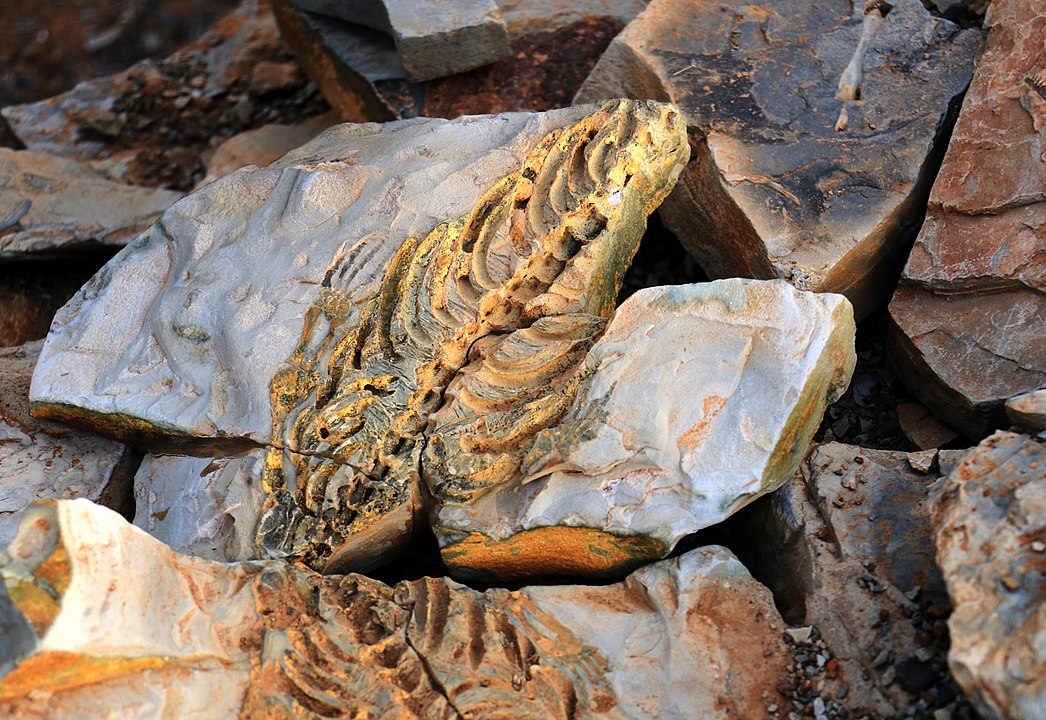
Photo by Olga Ernst & Hp. Baumeler, via Wikimedia.
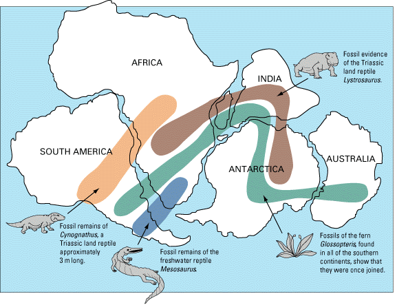
He highlighted a land plant and an aquatic (freshwater) reptile as two particularly useful examples. The reptile was Mesosaurus, known from two places on the planet: Brazil’s Paraná basin, and the Aranos basin of southwest Africa. When the position of the South American and African continents was reconstructed to their pre-Atlantic position, this created a cluster of Mesosaurus fossils sites that overlapped both continents.
Wegener realized there were three plausible ways of explaining this distribution. Consider these multiple competing hypotheses:
-
- The fossils represent two populations of the same species that got established in two continental locations thousands of kilometers apart, and somehow the original population surmounted the obstacle of the Atlantic Ocean to colonize the second location. Maybe the Mesosaurus scrabbled over there on a long skinny transatlantic land bridge, now eroded away? In this case, the continents don’t need to drift.
- The two groups of Mesosaurus fossils are an example of convergent evolution, independently derived on the two continents, and don’t actually represent a single ancestral population. In this case, the continents don’t need to drift.
- There was one population of Mesosaurus, established within the Pangaean supercontinent, and when Pangaea broke up, the continent of Africa drifted away from the continent of South America, splitting the Mesosaurus collection in two. In this case, the simplest story for the fossil distribution ends up implying something huge about the way the Earth works: continents drift!
Wegener, of course, opted for the final hypothesis.
The plant was a seed fern [Update link seed fern case study], Glossopteris. Here is a GIGAmacro view of some Glossopteris leaves – Zoom in to see their details:
GIGAmacro by Robin Rohrback.
USGS map.
Glossopteris has a late Paleozoic distribution across all the southern portion of Pangaea; what’s sometimes called Gondwana. Fossils of Glossopteris have been found in South America, Africa, Madagascar, Antarctica, India, and Australia. How best to explain this distribution? The same multiple working hypotheses that applied to Mesosaurus apply to Glossopteris, and again, Wegener found the “one population of Glossopteris, ripped asunder into six pieces by continental drift” the most compelling explanation.
Many other Permian-aged species show this same pattern, suggesting the timing for Pangaea’s existence.
Did I get it?
Landing with a thud
Though this evidence may seem compelling to us today, reception to Wegener’s proposal was mixed. Some prominent geologists east of the Atlantic championed the idea (notably Arthur Holmes in the United Kingdom and Alexander du Toit in South Africa), but it was a hard sell to American geologists. Wegener himself brought this paradigm-shifting idea to geology from outside the field; he was a meteorologist by training. Though that shouldn’t matter, it did. Scientists are people, and there is frequently a tendency to discount a radical idea offered by someone with less formal training that yourself. They waved off his compilation of evidence as mere coincidence, or sought to explain it by other means (the fossil distributions could be explained by since-vanished land bridges, for instance).
Public domain.
Wegener also made some calculations about the rate of continental movement, and got speeds that were two orders of magnitude faster than reality. Though geologists of his day had no clue what the real rate was, they did know that Wegener’s rate of 2.5 m/year seemed outrageously zippy. (For contrast, modern estimates of Atlantic Ocean divergence are ~2.5 cm/year.)
The fatal flaw though was that Wegener only documented evidence that the continents had moved. He did not take the idea further into a model for why they moved. Wegener did not suggest how they might have moved, only that they had. Did the continents plow through the ocean basins like icebreakers crossing a frozen lake? If so, what would compel them to do so? The lack of a conceivable driving mechanism for the horizontal movement of continents led most American geologists to reject the notion outright.
It is worth noting that Arthur Holmes did suggest mantle convection as a driver, as early as 1919. He even suggested a “bulge” where warm mantle material rose beneath the seafloor, presaging insights that would come in the 1950s and 1960s. But even this failed to overcome skepticism in the scientific community.
Finally, there was as yet no way to reconstruct the path a continent had taken through time, so a vital test was lacking. Technology would eventually catch up (paleomagnetism; see below), but too late for Wegener to be vindicated while he was alive. The idea was shelved, and when Wegener was killed on a meteorological expedition in Greenland in 1930, continental drift lost its most effusive champion.
Did I get it?
Other supercontinents
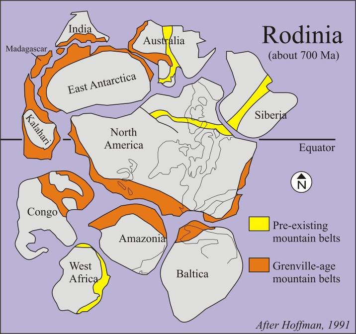
Callan Bentley graphic after an original by Paul Hoffman.
A brief note: We now know that Pangaea was not the only supercontinent, merely the most recent. Over the course of geologic history, continents have joined up into larger landmasses, and broken apart again repeatedly. We have a pretty clear view of Pangaea’s size and shape because that view is only sullied by its breakup. Earlier supercontinents are harder to make out, since each successive tectonic episode tends to overprint evidence of its predecessors. The various processes of “the rock cycle” (weathering and erosion, metamorphism, melting) tend to destroy older rocks, or modify them in ways that obscure the information that they previously carried within them. Nonetheless, we’ve been able to make out previous supercontinents, the more recent ones clearer than than the more ancient ones. There was Rodinia (~1 Ga), Nuna (~1.8 Ga), Ur (~2.6 Ga), and several others.
Did I get it?
Seafloor spreading
Wegener’s catalog of evidence for the past motion of the continents was revitalized when a new context was offered in the aftermath of World War II. The new context shifted the focus from the continents (~30% of the planet’s surface) to the rocks that floor the ocean basins (~70% of Earth’s surface). The new idea was that the seafloor was an ephemeral entity, forming at oceanic ridge systems, and destroyed elsewhere through the process of subduction.
The shape of the ocean basins
World War II was fought on many fronts. The relevant aspect of the conflict for the current discussion is submarine warfare. The United States Navy fought the German U-boats in the Atlantic Ocean, attempting to prevent tragedies like the sinking of the Lusitania. To aid in the war effort, sonar was utilized to map the seafloor to a greater degree than had previously been accomplished. When the data was declassified after the war ended, it revealed a fascinating aspect of the planet that had previously been hidden: the seafloor wasn’t flat!
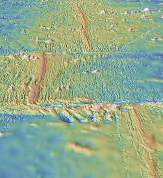
Visualization via GeoMapApp.
Instead, the longest range of mountains on the planet, the oceanic ridge system, wrapped around the planet much like the seams wrap around a baseball. Even the stitching on the baseball is relevant here, as it evokes the fracture zones that emanate from the ridge, perpendicular to the ridge’s trend. And right there are the crest of this odd ridge system was a valley, a rift valley. It looked like a scar.
The oceanic ridge system is 70,000 km (43,000 miles) long. In both the Atlantic and Indian Ocean basins, the ridges were in the middle of the ocean, equidistant from the continents on either side. This led many geoscientists to adopt the term “mid-ocean ridge” to describe them, but it’s worth noting that the East Pacific Rise is not in the middle of the Pacific Ocean. So oceanic ridge is the more inclusive term.
“Discovering Plate Boundaries” topography/bathymetry map by Dale Sawyer
There were also very deep spots in the ocean – long furrows that were quickly dubbed “trenches.” Curiously, these trenches paralleled chains of active volcanoes, and were in areas known to have lots of earthquakes.
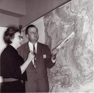
At Columbia Lamont-Doherty Earth Observatory, Bruce Heezen and Marie Tharp collaborated on detailed mapping of the seafloor, systematically constraining the variation in bathymetry with a series of profiles. They are celebrated today not only for their meticulous measurements, but because of a landmark visualization of these findings; they commissioned artist Heinrich Berann to paint a rendition of their seafloor map that popped in a way few scientific visualizations have ever matched. The finalized Heezen & Tharp map (with labels, etc.) was published in 1978.
Painting by Heinrich Berann, via the Library of Congress
How to explain this exciting new information about the shape of the largest region on our world?
An essay in geopoetry
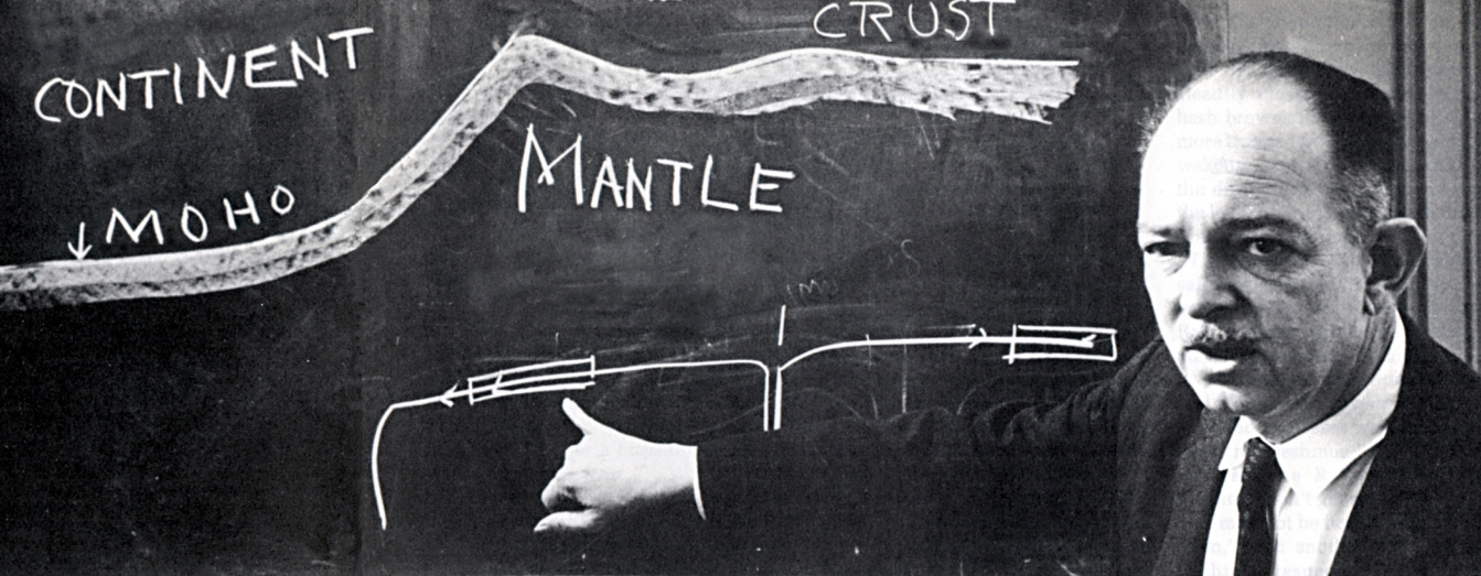
Harry Hess was a a geophysicist on the faculty at Princeton, and served as a captain in the United States Navy during World War II. He had experience with seafloor mapping using sonar on his own ship, and was deeply impressed with the Heezen & Tharpe ridge-top rift data when Heezen presented it at a departmental seminar in 1957. Hess’s paper outlined the case to be made that new seafloor was generated at the ocean ridges: that active spreading at those sites triggered magmatism that sealed the crack shut with new seafloor. But Hess went further: he didn’t think the planet was getting larger over time through ever-expanding ocean basins, but thought instead that a steady state ocean coverage could be maintained if some seafloor was recycled into the “jaw crusher” (his phrase) of the newly discovered oceanic trenches. Alpine geologist André Amstutz called these subduction zones, and though he wrote in French, the name was soon adopted in geoEnglish, too. Powering it all was convection in the underlying mantle: warm (but solid) rock rising beneath the oceanic ridges, and cold rock sinking beneath the subduction zones. Hess was conscious of how revolutionary these ideas were, and he modestly covered up the audaciousness of seafloor spreading by hedging his bet with self-deprecating humor. He waved his arms, and called his paper “an essay in geopoetry.”
Modified from an original by KDS4444.
Hess need not have been so coy; his ideas have been validated ever since. The seafloor spreads, adding new oceanic crustal material (basalt and gabbro) at the oceanic ridge system into the gap between diverging continents. Old oceanic crust is destroyed through subduction at deep sea trenches.
Did I get it?
Age of the oceanic crust
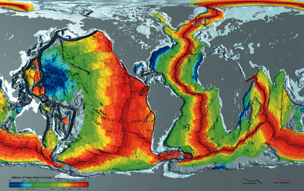
NOAA map.
Oceanographic expeditions such as the Deep Sea Drilling Program sampled the seafloor in many places, gathering cores of seafloor sediment down to the top of the oceanic crust. The age of the oldest sediment could be deduced through study of the microfossils it contained, and that would constrain the age of the crust beneath to be older. Scientists then used correlation with key features of the seafloor (ridges, fracture zones, etc.) to extend points where the age of the oceanic crust was known to cover wider regions. The overall pattern was that the youngest crust was located atop the oceanic ridges, and it got older perpendicular to the ridge, in both directions. In the Atlantic Ocean, for instance, the pattern offered a beautiful symmetry, with crust of 0 Ma age at the Mid-Atlantic Ridge, and Jurassic (~180 Ma) oceanic crust immediately adjacent to the North American and African continental shelves.
Did I get it?
Paleomagnetism
Like many planets, Earth generates its own magnetic field. This magnetic field manifests from flow of a magnetically-conductive fluid: the molten iron/nickel alloy of the outer core. What happens in the core doesn’t stay in the core: the magnetic field penetrates the mantle, crust, oceans, and atmosphere, and extends far out into space. This protects our planet from the atmosphere-eroding effects of the solar wind.
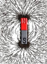
Closer to the surface, where rocks form that can later be studied by historical geologists, the magnetic field also makes an impression. Certain minerals are magnetically sensitive. There are several, including ilmenite and hematite, but for our purposes here, let’s focus on magnetite. Crystals of magnetite have freedom of movement within a molten lava flow or within a body of sediment settling through a water column. Given the freedom to move, they will rotate into alignment with Earth’s prevailing magnetic field. When the rest of the surrounding lava is crystallized, or when the surrounding sediment is lithified, the grains of magnetite are no longer free to move. At this point, they are “fossil” evidence of Earth’s magnetic field, and if they are moved to new locations, or new orientations, they take their “stamp” of the old magnetic field with them. We call the study of old magnetic orientations paleomagnetism.
Geophysicists who study paleomagnetism (who cheekily call themselves “paleomagicians”) collect very precisely oriented samples of magnetite-bearing igneous or sedimentary rocks and bring them back to a lab where a well-shielded magnetometer measures the remnant magnetism.
Inclination
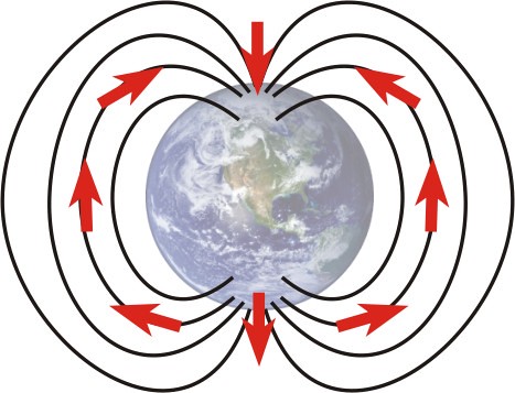
Callan Bentley illustration.
Latitude on Earth today (position on Earth’s surface between the Equator and the poles) corresponds strongly with the inclination of Earth’s magnetic field. The lines of magnetic force emanate from the South magnetic pole, wrap around the planet, and dive back into the planet at the North magnetic pole. The lines are vertical at these polar locations (i.e., perpendicular to Earth’s surface), but horizontal at the magnetic Equator (i.e., parallel to Earth’s surface).
To interpret paleolatitude, we apply this modern observation to the past through the lens of uniformitarianism. If we find a sedimentary rock layer with magnetite crystals that show a bedding-perpendicular orientation, we would infer a polar latitude of origin for the original sedimentary deposit. (We apply the principle of original horizontality to infer the bed was laid down more or less horizontally, so a bedding-perpendicular paleomagnetic inclination means “vertical” when it formed.) Conversely, if we find a sedimentary rock layer bearing magnetite crystals that have their magnetic orientation parallel to the bed, then that would imply the sediment was deposited near the paleomagnetic Equator. Intermediate latitudes have values that are intermediate between horizontal and vertical, and the variation occurs in a systematic way.
Declination
Now consider another behavior of a free-spinning magnet in a magnetic field: a compass needle. Like a crystal of magnetite, the compass needle is magnetically susceptible, and will align itself with the planet’s magnetic field, pointing toward magnetic north. Fossil magnets pull this same trick. We call the variation between a given direction and north by the name declination. If you want to track how a given landmass has moved through geologic time, paleomagnetic declination comes in handy. In this case, you want a sequence of sedimentary strata and/or lava flows, spanning the relevant portion of geologic time. If you are successfully in extracting paleomagnetic declination information from them, and you can successfully constrain the ages of the layers, you will get a series of time-stamped declination directions. For instance:
| 500 Ma | “The north magnetic pole was at 190° to the modern north pole, at a latitude distance of 40°.” |
| 350 Ma | “The north magnetic pole was at 230° to the modern north pole, at a latitude distance of 60°.” |
| 200 Ma | “The north magnetic pole was at 300° to the modern north pole, at a latitude distance of 80°.” |
| 50 Ma | “The north magnetic pole was at 350° to the modern north pole, at a latitude distance of 100°.” |
In this hypothetical example, four dates/orientations spanning half a billion years constrain the movement of that block of crust increasingly southward (crossing the equator sometime between 200 Ma and 50 Ma), and rotating clockwise all the while.
This “testimony” from the strata of a given location is called an apparent polar wander path. It is basically how one particular spot on a given continent might view the north magnetic pole through time.

Callan Bentley graphic, after an original from Geotimes.
But different continents tell different stories – they have apparent polar wander paths that do not make any sense if the continents are eternally fixed in place. If continents were not permitted to drift, then the implication from a half dozen different continents’ apparent polar wander paths is that in the past there were numerous magnetic north poles, arrayed all over the place, and over geologic time they have gotten closer to the modern north pole, and merged into one. This makes no sense, in terms of what we know about how magnets work. But, if the continents are free to drift, and the seafloor to spread in between them, or subduct in front of them, suddenly you only need one planetary magnetic field to make sense of the continents’ plurality of parochial perspectives.
In other words, paleomagnetic inclination gives us a way to quantify the past motion of a given plate (continent) relative to a more or less stationary magnetic north pole.
Polarity reversals

Public domain via Wikimedia.
The final aspect of paleomagnetism that bears consideration has to do with reversals of the magnetic field. We’ve previously discussed (a) inclination and (b) declination as being related to angles between a line of magnetic force and (a) Earth’s surface and (b) the direction to the north pole. But that line is not just a line; it is an arrow. In other words, all lines of magnetic orientation have a direction to them – a direction in which they point. A rock forming at the modern day south pole would have a vertical magnetic inclination, but so would one forming at the north pole. How can we tell them apart? Earth’s magnetic flow exits the planet at the south magnetic pole and re-enters at the north magnetic pole. So the modern South Pole rock would have an arrow pointing “up” (away from Earth’s surface), while the modern North Pole rock would have an arrow pointing “down” (toward Earth’s interior).
By paying attention to which way these arrows point, we arrive at an interesting insight: they frequently switch back and forth! The reason why these reversals happen is not entirely clear, but it is plain that they do — and we can use that to our advantage. Not only does it open up a whole new avenue for dating rocks (reading their “magnetostratigraphy” like a bar code) but it also provides a tool for confirming that seafloor spreading is, in fact, real.
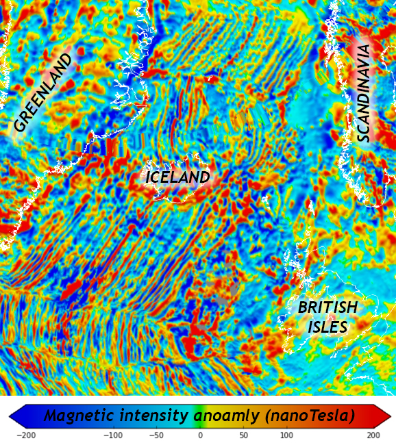
Modified from a presentation of the EMAG2 model by Maus, et al. (2009).
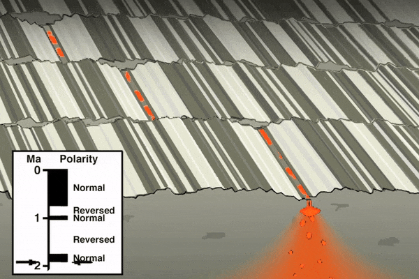
When new oceanic crust is generated, magma wells up from the mantle below, where it is produced through decompression partial melting. Within that magma are magnetically-susceptible minerals (like magnetite). The magma injects into the crack between the two diverging plates, and solidifies. At that moment, the magnetic signature of that moment in Earth history is locked into the plate. Then tensional stresses build up anew, the crust cracks again, and more magma squirts in to seal it shut, again, taking on the magnetic signature of the Earth. If a reversal happened in between dike-injection events, that will be preserved as “stripes” of oppositely-oriented magnetism on the seafloor — something that we can readily measure using a submersible magnetometer towed behind a ship.
It turns out that the pattern of magnetic reversals in Earth’s oceanic crust is recorded twice – once in each direction leading away from the oceanic ridge system. This is a prediction of the Vine-Matthews-Morley hypothesis (named for three geophysicists who suggested it):
Animation by Tanya Atwater, UCSB.
Paleomagnetic stripes in the seafloor are like a doubly-redundant tape recording of the reversals in Earth’s magnetic field. The “normal” polarity of the Bruhnes chron that we are currently in can be found astride the ridges all over the world, but head a short distance away (in either direction) and you’ll soon encounter the “reversed” signature of the older Matuyama chron. The two records are like mirror images of one another.
These patterns of magnetic “stripes” parallel to the oceanic ridge system and faithfully recording the changes in the planet’s magnetic polarity were perhaps the most compelling line of evidence yet in support of seafloor spreading, and thus plate tectonics.
Did I get it?
Hot spot tracks
Remember that one of the errors Alfred Wegener made was to estimate too-fast rates of speeds for his drifting continents. Now that the idea of seafloor spreading had been established, a test could be made. Numerical dating of igneous rocks had become validated as a technique during the interregnum between Wegener’s book and Hess’s paper, and attention soon turned to island archipelagos such as Hawaii and the Galapagos.
Callan Bentley photo.
Unlike volcanic island arcs, which feature a trench-parallel line of volcanoes all erupting at various times, on and off, over and over, Hawaii and the Galapagos are different. In each archipelago, the volcanoes show an age progression. At one end of the chain is an active volcano or two, erupting lava and ash in the present day. But as you work your way toward the other end of the chain, the volcanoes are inactive and more weathered. Sure enough, radiometric dating confirms our suspicion: they get older in one direction! In Hawaii, the volcanoes get older toward the northwest. In the Galapagos, the volcanoes get older toward the east. One explanation that has been offered to explain this age progression is that there is a source of magma unrelated to plate tectonics, piercing upward periodically with injections of magma as the plate of oceanic lithosphere moves steadily overhead. This simple notion has a simple name: it’s a hot spot.
Hot spot volcanism implies that if a plate, such as the Pacific Plate, is moving at a steady rate in a given direction over a stationary hot spot, periodically magma from the hot spot will burst through, making volcanoes on the surface of the plate, which will then trundle them along, away from the hot spot. The volcano will go dormant, begin to weather and erode, and will subside. To the northwest of the main Hawaiian islands are a series of seamounts: not nearly as much landmass pokes up above sea level, but they still represent a massive bump on the face of the Pacific Plate. Advocates of the hot spot interpretation for Hawaii would interpret these seamounts as places that used to be on top of the hot spot, but have long since been dragged away.
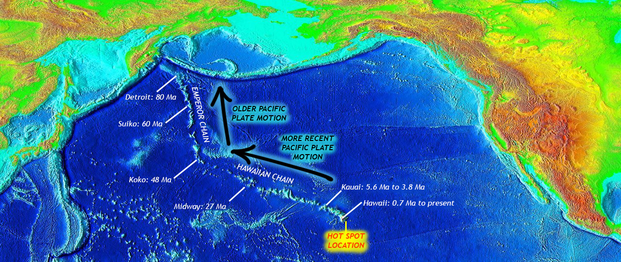
Callan Bentley modification of USGS map.
A kink in the seamount chain can be found northwest of the Midway Atoll, where the Emperor Seamount chain trends off toward the north. This reflects a change in direction of the Pacific Plate that took place around 48 Ma.
The Pacific is a fast-moving plate. In some places, it’s moving about 10 cm/year relative to a fixed frame of reference. Plates can dawdle along at a slower pace, too; For instance, the Atlantic is widening at only 2.5 cm/year. Even a fast moving plate is still too slow for the human eye to perceive. We frequently liken the pace of plate movement to the rate of fingernail growth. You can’t see it happen, but you know it happens. I suppose nail clippers are the subduction zone in that analogy…
Did I get it?
Conclusion
Scientific understanding proceeds erratically. Alfred Wegener’s attention to the continents was valuable, but wasn’t capable of achieving intellectual liftoff on its own. Our understanding of Earth surface dynamics needed a shot in the arm – an infusion of fresh data. When geophysical surveys of the ocean basins were revealed in the aftermath of a great global conflict, seafloor spreading was born. The new idea about the ocean basins was mixed with continental drift to yield the theory of plate tectonics.
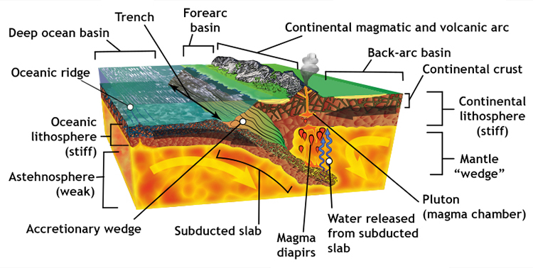
Plate tectonics says that the outermost rocky surface of our planet is broken into a series of slabs called “plates.” These plates may be made of continental lithosphere, oceanic lithosphere, or (usually) both. The plates move around, and the action that occurs at their boundaries (convergent, divergent, and transform) are vital in producing a suite of major geological phenomena: mountain belts, volcanic arcs, deep sea trenches, oceanic ridges, rift valleys, laterally offset geologic units and belts of earthquake activity.
Now you have a sense of the scientific history of this important idea. But plate tectonics isn’t stuck in the 1960s. The past half a century has repeatedly tested and refined our understanding of the behavior of Earth’s lithosphere, leading to great insights in Historical Geology. If you haven’t already read it, it’s now time to examine the discussion of modern plate tectonics.
Further reading
Callan Bentley (2017). “Travels in Geology: Geo-diversity and geologic history in the North West Highlands of Scotland,” EARTH magazine, May 2017.
Heinrich C. Berann, Bruce C. Heezen, and Marie Tharp. Manuscript painting of Heezen-Tharp “World ocean floor” map. [1977] Map.
Hali Felt (2012). Soundings: The Story of the Remarkable Woman Who Mapped the Ocean Floor. Henry Holt and Co., 352 pages.
Harry Hess (1962). “History of Ocean Basins,” chapter in Petrologic Studies: A volume in honor of A.F. Buddington. Geological Society of America.
S. Maus, U. Barckhausen, H. Berkenbosch, N. Bournas, J. Brozena, V. Childers, F. Dostaler, J. D. Fairhead, C. Finn, R. R. B. von Frese, C. Gaina, S. Golynsky, R. Kucks, H. Lühr, P. Milligan, S. Mogren, R. D. Müller, O. Olesen, M. Pilkington, R. Saltus, B. Schreckenberger, E. Thébault, and F. Caratori Tontini (2009). “EMAG2: A 2-arc min resolution Earth Magnetic Anomaly Grid compiled from satellite, airborne, and marine magnetic measurements,” Geochemistry, Geophysics, Geosystems 10, Q08005, doi:10.1029/2009GC002471.
Ted Nield (2007). Supercontinent. Granta Books, 352 pages.
Naomi Oreskes (1999). The rejection of continental drift. Oxford University Press, 432 pages.
Chris Johnson, Matthew D. Affolter, Paul Inkenbrandt, & Cam Mosher (2017). “Plate tectonics,” An Introduction to Geology, OER textbook: CC-BY.
Alfred Wegener (1929), translated by John Biram (1966). The origin of continents and oceans. Dover Publications, Inc., 246 pages.