5 – Optical Mineralogy

KEY CONCEPTS

• Light entering a crystal may be absorbed, refracted, or reflected.
• Optical mineralogy involves studying rocks and minerals by studying their optical properties.
• Today, most optical mineralogy involves examining thin sections with a petrographic microscope.
• Petrographic microscopes have polarized light sources that illuminate a thin section.
• We examine thin sections in two modes: using plane-polarized light or using cross-polarized light.
• In plane-polarized light we can distinguish opaque and nonopaque minerals; we can see crystal shape, habit, cleavage, color and pleochroism, and relief.
• In cross-polarized light, we distinguish anisotropic from isotropic minerals, we see interference colors related to birefringence, and we can see twinning and related features.
• We use cross-polarized light to learn a crystal’s optic class and optic sign, to measure extinction angles and sign of elongation, and to measure 2V.
• A combination of optical properties allows us to identify minerals in thin section and to interpret geologic histories.

● Box 5-1   For an Alternative Approach This chapter contains the standard and fundamental information about optical mineralogy. But there are many ways to approach this topic. For an alternative approach, and to see many excellent videos, go to “Introduction to Petrology” by Johnson, E.A., Liu, J. C., and Peale, M. at: https://viva.pressbooks.pub/petrology

● Box 5-2   Prologue: An Introduction to Optical Mineralogy The principles of optical mineralogy and mineral microscopy can be confusing. A standard approach into complicated science topics is to start with a discussion of underlying principles and to build to more complicated concepts. And we will do that. But because mineral optics can seem arcane, before we jump into the underlying fundamentals, we will begin with a video that gives some background and a broad overview without all the details of optical theory and microscopy. The video finishes up by discussing the most important aspect of optical mineralogy, which is viewing rocks and minerals in thin section. And everything that follows this box in Chapter 5 is building to that end. ▶️ Video 1: An Introduction to Optical Mineralogy (9 minutes)

5.1 Introduction to Mineral Optics

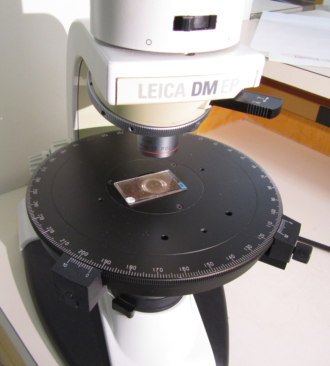
Optical mineralogy involves studying rocks and minerals by studying their optical properties. Some of these properties are macroscopic and we can see them in mineral hand specimens. But generally we use a petrographic microscope, also called a polarizing microscope (Figures 5.1 and 5.2 show examples), and the technique is called transmitted light microscopy or polarized light microscopy (PLM). A fundamental principle of PLM is that most minerals – even dark-colored minerals and others that appear opaque in hand specimens – transmit light if they are thin enough. In standard petrographic microscopes, polarized light from a source beneath the microscope stage passes through samples on the stage and then to your eye(s).

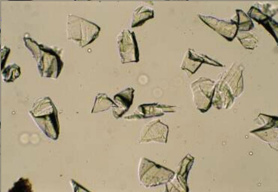
One approach to PLM involves examining grain mounts, which are ground-up mineral crystals on a glass slide. The grains must be thin enough so that light can pass through them without a significant loss of intensity, usually 0.10 to 0.15 mm thick. We surround a small number of grains with a liquid called refractive index oil, and then place a thin piece of glass, called a cover slip, over the grains and liquid. The photo in Figure 5.3, below, shows garnet grains in a grain mount.

Grain mounts and refractive index oils are necessary for making some types of measurements, but are not the focus of this chapter. They were extensively used in the past, but are not much used today. For more detailed information about studying minerals in grain mounts consult an optical mineralogy textbook.

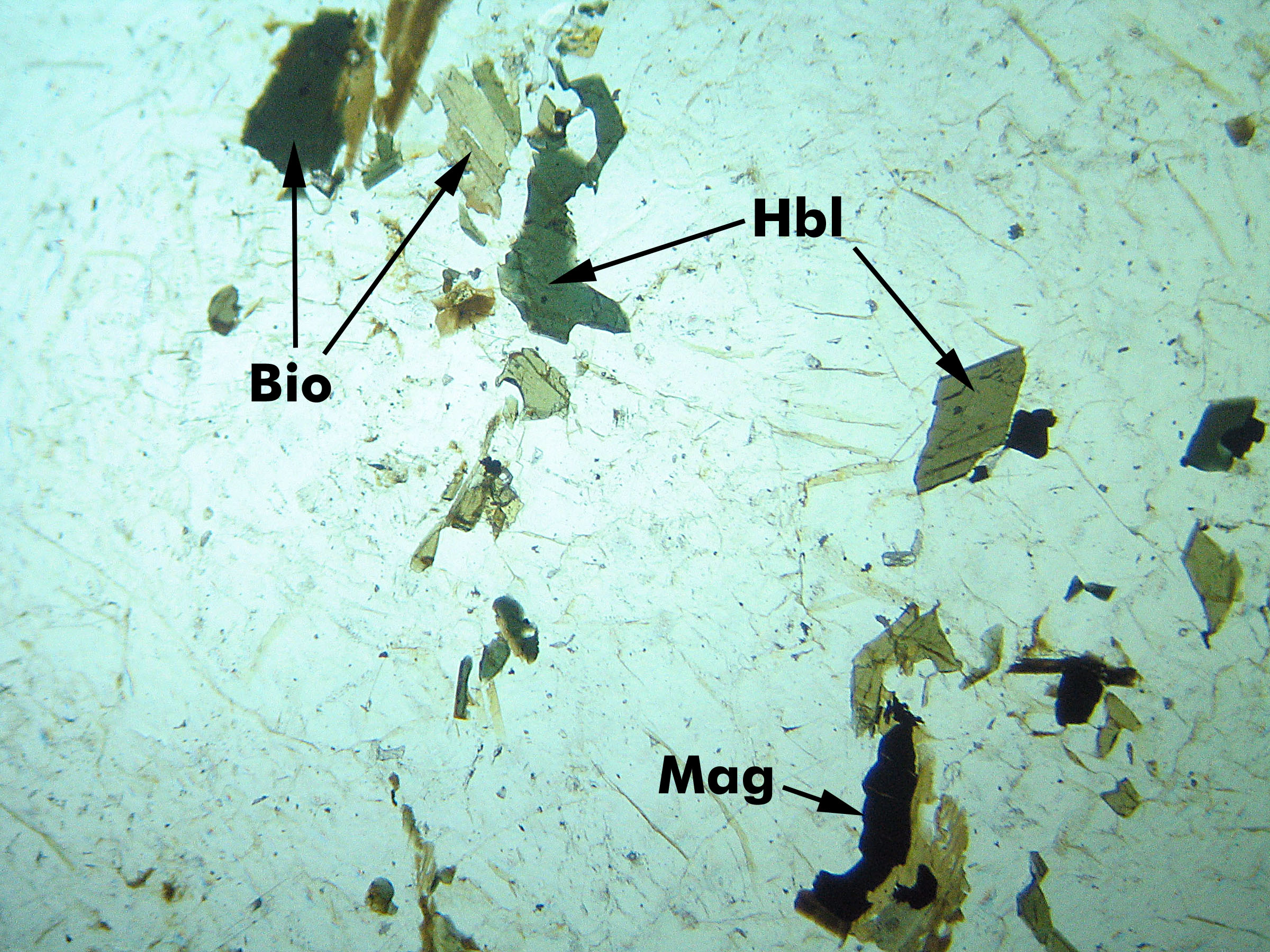
Most optical mineralogy today involves specially prepared thin sections (0.03-mm-thick specimens of minerals or rocks mounted on glass slides). Video 1 (linked in Box 5-2) explains how we make thin sections, and Figure 5.1, the opening figure in this chapter, shows an example. Figure 5.4 above shows a microscope view of a thin section that contains several minerals (biotite, hornblende, and magnetite are labeled, and the clear grains around them are mostly quartz and plagioclase). Whether looking at grain mounts or thin sections, transmitted light microscopy allows us to determine and measure properties that are otherwise not discernible. We can identify minerals, sometimes their compositions, and we can observe mineral relationships that allow us to learn about mineral origins.

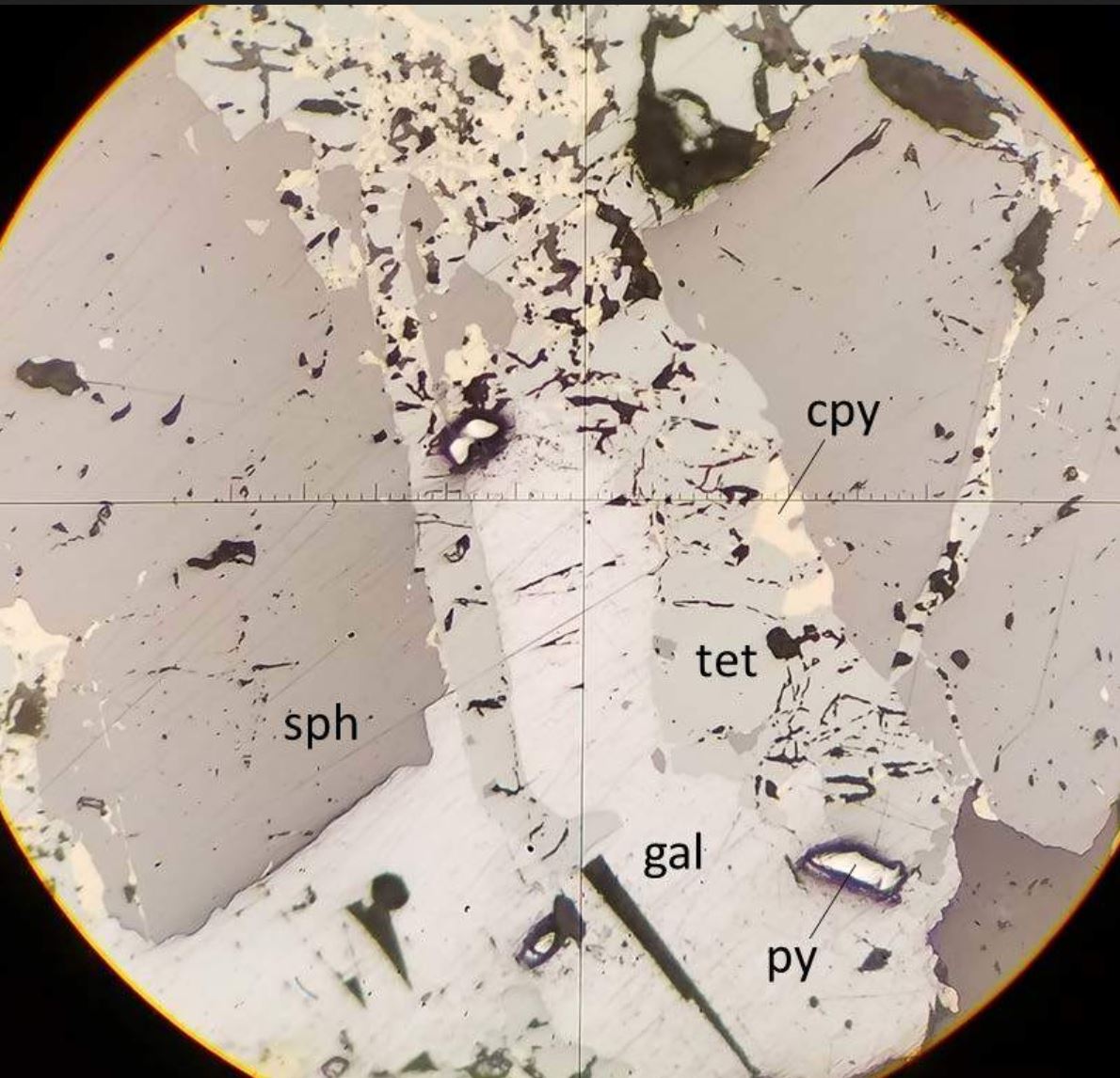
Minerals with metallic luster and a few others are termed opaque minerals. They will not transmit light even if they are thin-section thickness. So they always appear black when viewed with a microscope. Magnetite is an opaque mineral; the photo in Figure 5.4 contains several small black magnetite grains. For studying opaque minerals, transmitted light microscopy is of little use. Reflected light microscopy (RLM), a related technique, can reveal some of the same properties. As the name implies, when using RLM, the light source is above the sample and light reflects from the sample to our eye. RLM, although an important technique for economic geologists who deal with metallic ores, is not used by most mineralogists or petrologists. So we discuss it only briefly in this book. Figure 5.5 shows a view of ore from Butte, Montana, seen with a reflecting light microscope. It contains several opaque minerals: galena, sphalerite, pyrite, and chalcopyrite. They appear in various shades of black, gray, and light yellow.

Most minerals can be identified when examined with a petrographic microscope, even if unidentifiable in hand specimen. Optical properties also allow a mineralogist to estimate the composition of some minerals. For example, we can learn the magnesium-to-iron ratio of olivine, (Mg,Fe)₂SiO₄, based on optical properties. And we can also determine the albite and anorthite content of plagioclase feldspar.

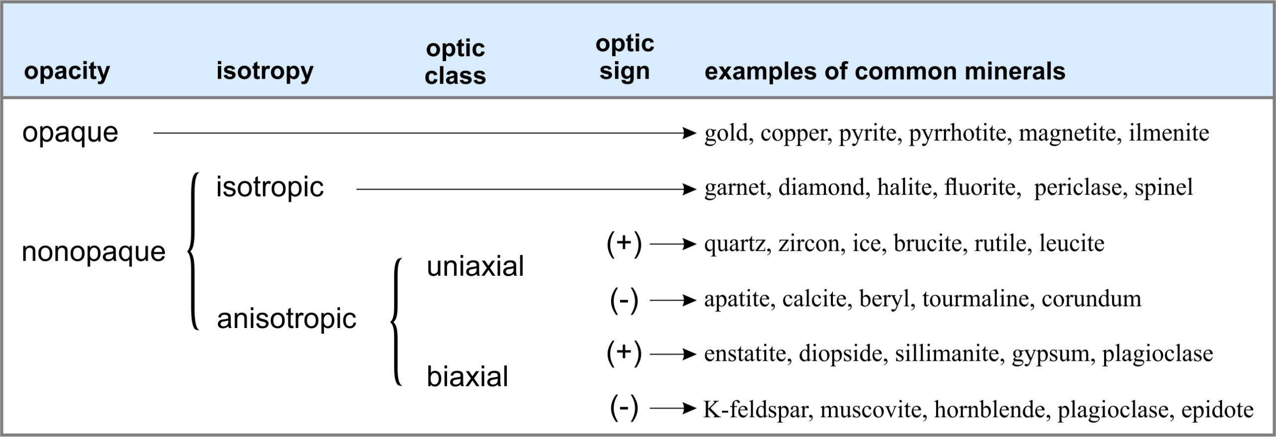
Box 5-3 (below) summarizes the optical properties used for mineral identification and gives the properties of some common minerals. At the largest level, we divide minerals into opaque minerals and nonopaque minerals. Opaque minerals will not transmit light unless the mineral grains are much thinner than normal thin sections. We further divide nonopaque minerals into those that are isotropic (having the same properties in all directions) and those that are anisotropic (having different optical properties in different directions). We discussed these terms, isotropic and anisotropic, previously in Section 4.1, Chapter 4. Finally, we divide the anisotropic minerals into those that are uniaxial and those that are biaxial, and according to whether they have a positive or negative optic sign. We look at the details of these and other diagnostic properties below.

Besides mineral identification, the polarizing microscope reveals important information about rock-forming processes (petrogenesis). When we examine thin sections, distinguishing igneous, sedimentary, and metamorphic rocks is often easier than when we look at hand specimens. More significantly, we can identify minerals and distinguish among different types of igneous, sedimentary, and metamorphic rocks. The microscope allows us to see textural relationships in a specimen that give clues about when and how different minerals in an igneous rock formed. Microscopic relationships between mineral grains allow us to determine the order in which minerals crystallized from a magma, and we can identify minerals produced by alteration or weathering long after the crystals first formed. Similar observations are possible for sedimentary or metamorphic rocks. Only the microscope can give us such information, information that is essential if rocks are to be used to interpret geological processes and environments.

● Box 5-3  Optical Classification of Minerals Mineralogists often classify minerals according to the mineral’s optical properties. The table below shows the basic classification scheme and gives examples of minerals belonging to each of six categories. At the highest level, we divide minerals into two groups: opaque minerals and nonopaque minerals. We further divide the nonopaque minerals into those that are isotropic and anisotropic, and then we divide the anisotropic minerals by other properties discussed later in this book. We measure these properties using a polarizing microscope such as the one in Figure 5.2 (above) and Figure 5.22 (later in this chapter).

5.2 Light and the Properties of Light

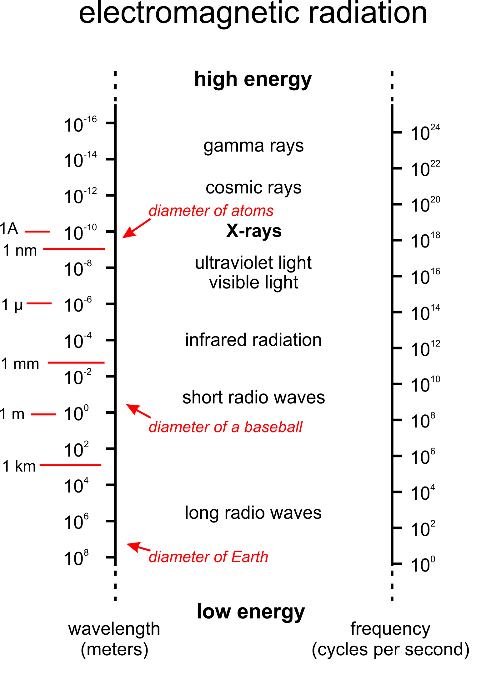
Before starting a discussion of optical mineralogy, it is helpful to take a closer look at light and its properties. Light is one form of electromagnetic radiation (Figure 5.6). Radio waves, ultraviolet light, and X-rays are other forms of electromagnetic radiation. All consist of propagating (moving through space) electric and magnetic waves (hence the term electromagnetic). The interactions between electric waves and crystals are normally much stronger than the interactions between magnetic waves and crystals (unless the crystals are magnetic). Consequently, this book only discusses the electrical waves of light. In principle, however, much of the discussion applies to the magnetic waves as well.

Because light waves have wavelengths two orders of magnitude greater than atom sizes or bond lengths, the interactions of light with crystals does not reveal information about individual atoms in a crystal. To obtain that kind of information, we must study crystals using shorter wavelength radiation, X-rays (Chapter 12).

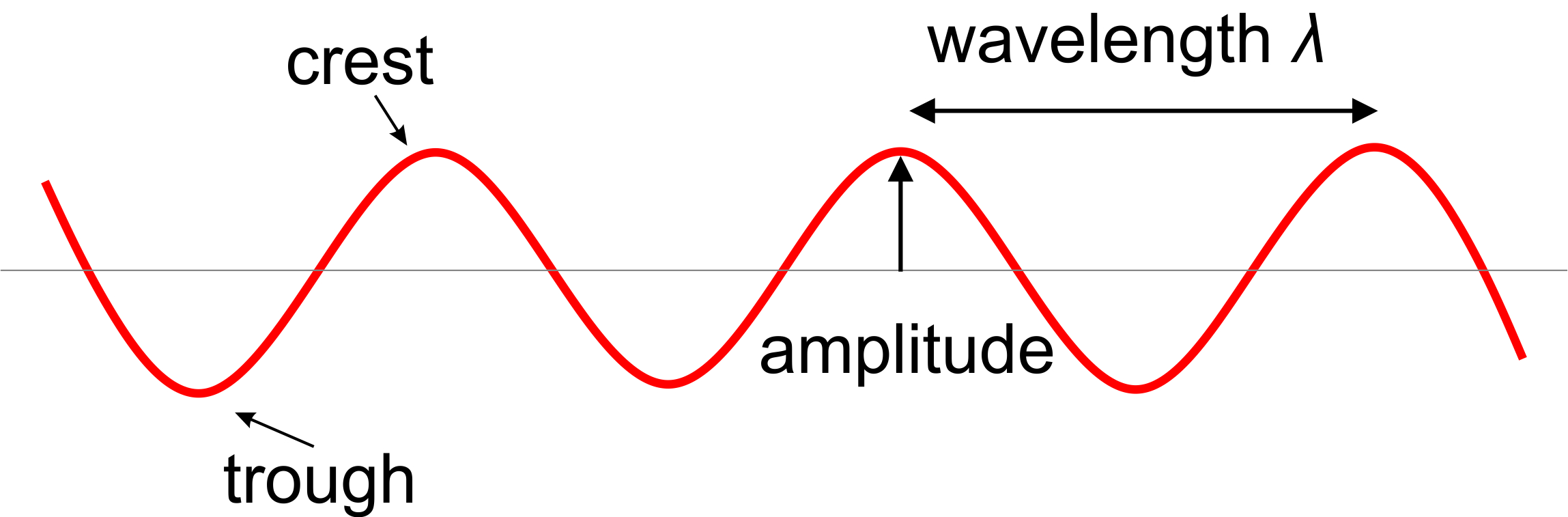
Light waves, like all electromagnetic radiation, are characterized by a wavelength, λ, and a frequency, ν (Figure 5.7). The velocity, v, of the wave is the product of λ and ν:
blankv = λν

In a vacuum, light velocity is 3 x 10⁸ meters per second. Velocity is slightly less when passing through air, and can be much less when passing through crystals. When the velocity of light is altered as it passes from one medium (for example, air) to another (perhaps a mineral), the wavelength changes, but the frequency remains the same.

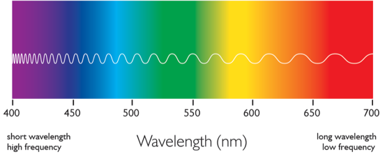
Visible light has wavelengths of 390 to 770 nm, which is equivalent to 3,900 to 7,700 Å, or 10^-6.1 to 10^-6.4 m. Different wavelengths correspond to different colors (Figure 5.8). The shortest wavelengths (violet light) grade into invisible ultraviolet radiation. The longest wavelengths, corresponding to red light, grade into invisible infrared radiation.

Light composed of multiple wavelengths appears as one color to the human eye. If wavelengths corresponding to all the primary colors are present with equal intensities, the light appears white. White light is said to be polychromatic (many colored), because it contains a range, or spectrum, of wavelengths. Polychromatic light can be separated into different wavelengths in many ways. When one wavelength is isolated, the light is monochromatic (single colored).

5.2.1 Interference

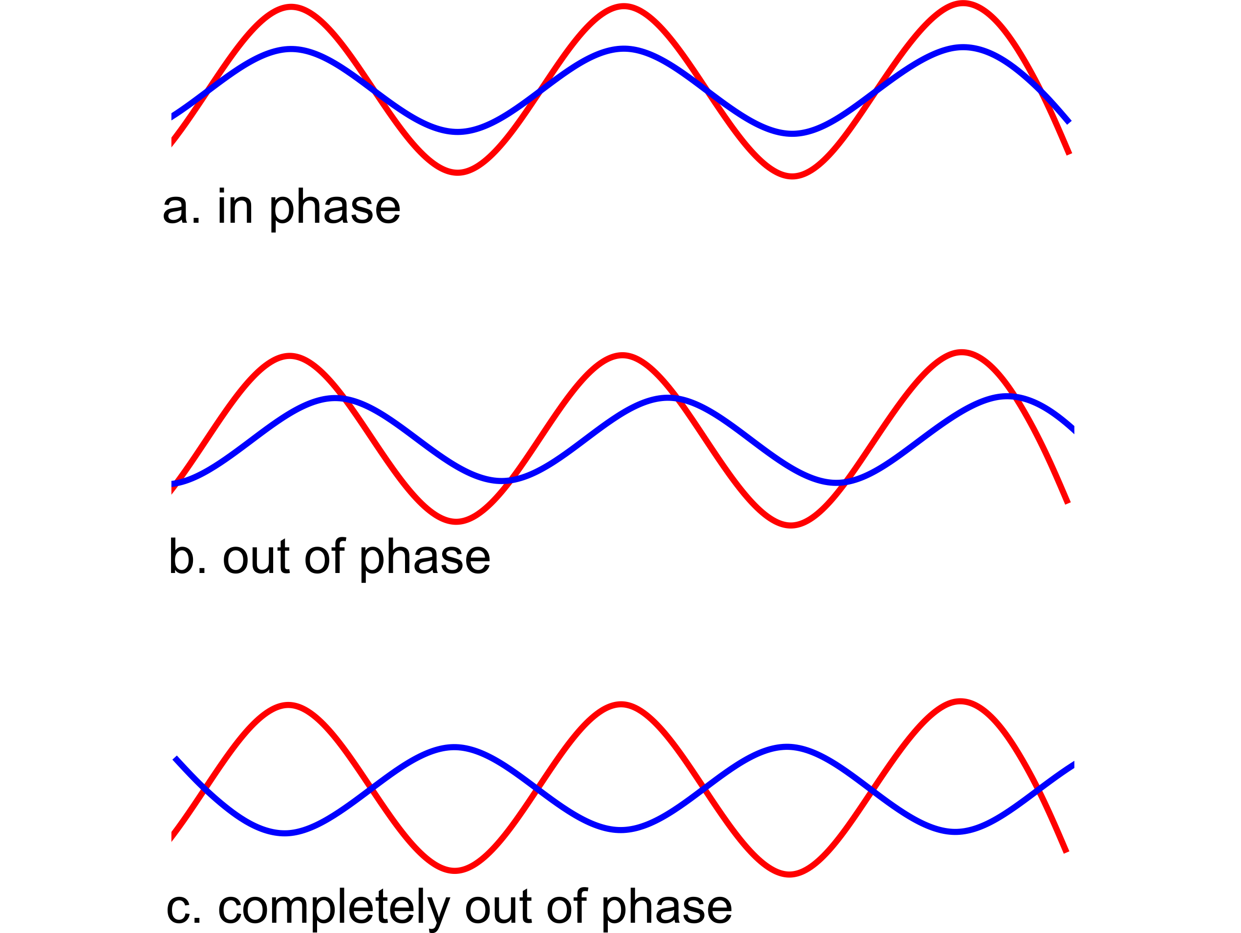
Besides wavelength (λ) and frequency (ν), an amplitude and a phase characterize all waves. Amplitude (A) refers to the height of a wave. Phase refers to whether a wave is moving up or down at a particular time. If two waves move up and down at same times, they are in phase; if not, they are out of phase.

When two waves with the same wavelength travel in the same direction simultaneously, they interfere with each other. Their amplitudes may add, cancel, or be somewhere between. The nature of the interference depends on the wavelengths, amplitudes, and phases of the two waves. Light waves passing through crystals can have a variety of wavelengths, amplitudes, and phases affected by atomic structure in different ways. They yield interference phenomena, giving minerals distinctive optical properties.

In Figure 5.9a, two in-phase waves of the same wavelength are going in the same direction. If we could measure the intensity of the two waves together, we would find that their amplitudes have added. When waves are in phase, no energy is lost; this is constructive interference. In contrast, Figure 5.9b shows two waves that are slightly out of phase, and Figure 5.9c shows two waves that are completely out of phase.

When waves are out of phase, wave peaks and valleys do not correspond. If they are completely out of phase, the peaks of one wave correspond to the valleys of the other. Consequently, addition of out-of-phase waves can result in destructive interference, a condition in which the waves appear to “consume” some or all of each other’s energy. (The First Law of Thermodynamics tells us that energy cannot disappear, so if two waves appear to cancel each other it means that the energy is going in another direction.) For perfect constructive or destructive interference to occur, waves must be of the same wavelength but they may have different amplitudes (as shown in Figure 5.9c). Interaction of waves with different wavelengths is much more complicated.

5.2.2 The Velocity of Light in Crystals and the Refractive Index

When light passes near an atom, perhaps in a crystal, the vibrating electric wave causes electrons orbiting the atom to oscillate. The oscillations absorb energy from the light, and the wave slows. As light passes from air into most nonopaque minerals, its velocity may decrease by a third or a half. Because the frequency of the light remains unchanged, we know that the wavelength must decrease by a similar fraction (because v = λν).

A wave’s velocity through a crystal is described by the crystal’s refractive index (n), which depends on chemical composition, crystal structure, and bond type in the crystal. The refractive index (n) is the ratio of the velocity (v) of light in a vacuum to the velocity in the crystal:
blankn = v_vacuum / v_crystal

Because light passes through a vacuum faster than through any other medium, n always has a value greater than 1. High values of n correspond to materials that transmit light slowly. Under normal conditions, the refractive index of air is 1.00029. Because it is much easier to work with air than with a vacuum, this is a common reference value and we often calculate refractive index as:
blankn = v_air / v_crystal

Refractive Index Values
air fresh water fluorite borax sodalite window glass quartz garnet zircon zincite diamond	1.000293 1.333 1.434 1.466 1.480 1.52 1.533 1.78 1.923 2.021 2.419

Most minerals have refractive indices between 1.5 and 2.0 (see examples in the table to the right). Fluorite, borax, and sodalite are examples of minerals that have a very low ( < 1.5) index of refraction. At the other extreme, zincite, diamond, and rutile have very high indices (> 2.0). The refractive index is one of the most useful properties for identifying minerals in grain mounts but is less valuable when we examine thin sections because it is impossible to determine precise values for n when viewing minerals in thin section.

 

 

5.2.2.1 Snell’s Law and Light Refraction

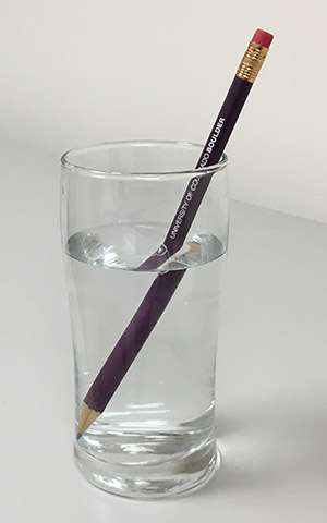
We have all seen objects that appear to bend as they pass from air into water. A straw in a glass of soda, or an oar in lake water, seem bent or displaced when we know they are not. We call this phenomenon refraction. Figure 5.10 shows an example – a pencil in a glass of water. Refraction occurs when light rays pass from one medium to another (for example water and air in Figure 5.10) with a different refractive index. If the light strikes the interface at an angle other than 90°, it changes direction and can distort a view. (Refraction occurs for waves of many different types, not just light waves. For example, earthquake waves are refracted as they interact with layers in Earth.)

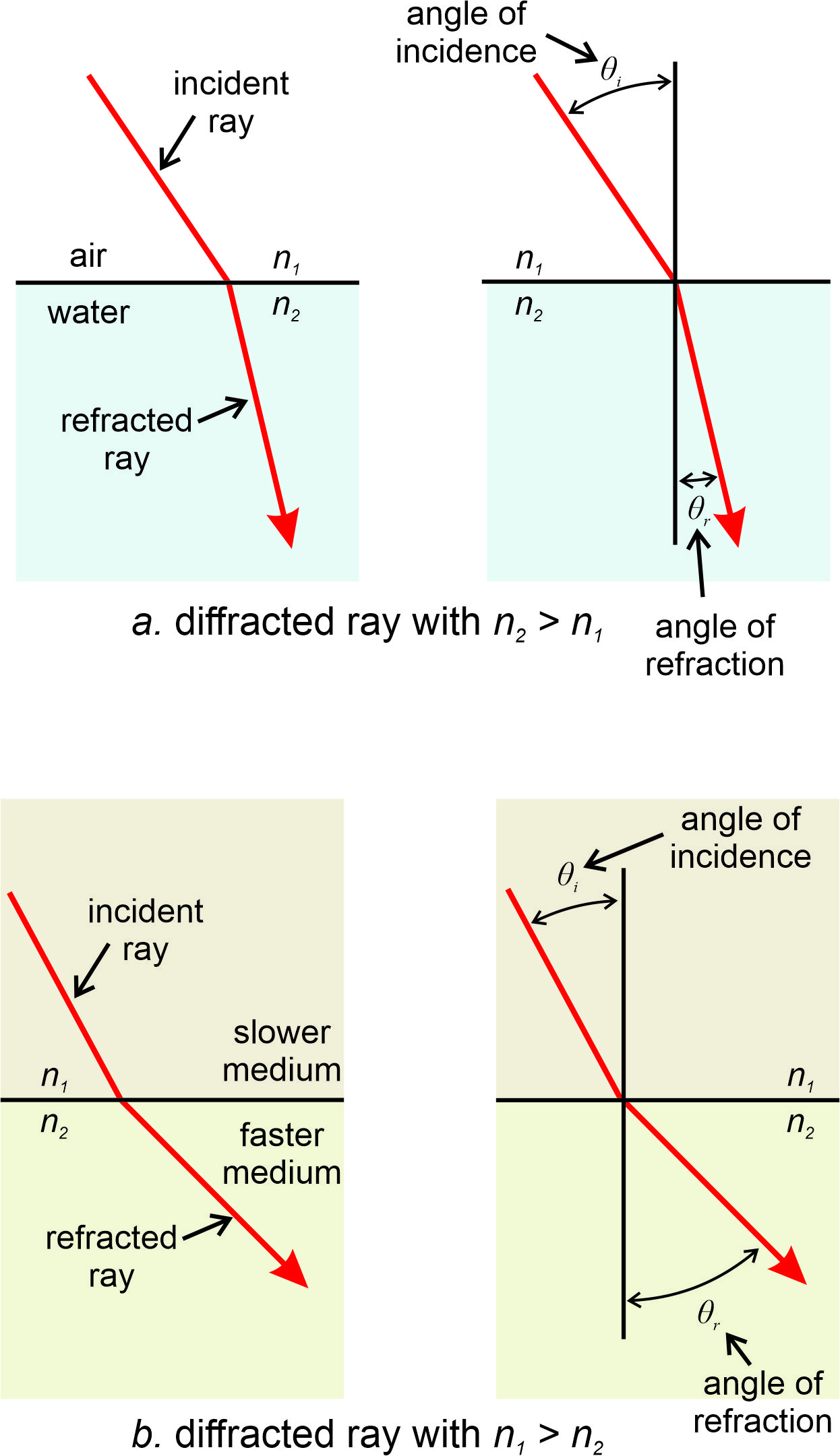
When refraction occurs, a light beam bends toward the medium with higher refractive index (where light travels slower) because one side of the beam moves faster than the other. Consider a beam traveling from air into water (Figure 5.11a). The side of the beam that reaches the interface first will be slowed as it enters the water. It sort of stubs its toe. So the beam bends toward the water. However, no refraction occurs for beams traveling at 90° to an interface between media with different refractive indices; the beam follows a straight course.

Figures 5.11b shows the opposite case: a beam traveling from a medium with a high refractive index (slower light velocity) into another with a lower refractive index (faster light velocity). The beam refracts toward the medium with a higher index, as it did in Figure 5.11a.

As seen in Figure 5.11, when light reaches an interface between two different media, the angle between the beam and a perpendicular to the interface is the angle of incidence (θ_i). After crossing the interface, the angle between the beam and a perpendicular to the interface is the angle of refraction (θ_r). The relationship between the angle of incidence (θ_i) and the angle of refraction (θ_r) is
blanksin(θ_i) / sin(θ_r) = v_i / v_r = n_r / n_i

where v_i and v_r are the velocities of light through two media, and n_i and n_r are the indices of refraction of the two media. This relationship, Snell’s Law, is named after Willebrod Snell, the Dutch scientist who first derived it in 1621.

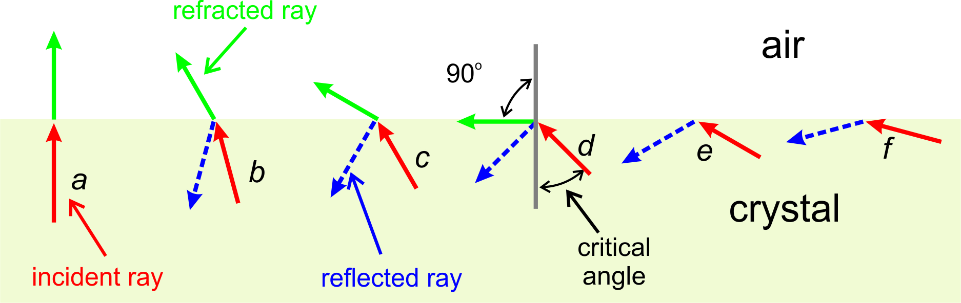
Figure 5.12 shows an incident light ray passing from within a crystal to air outside the crystal. If the incident ray is perpendicular to the crystal-air interface (drawing a), all light leaves the crystal. If the angle incidence is small (drawing b), most light escapes and is refracted at some angle to the crystal face, but some light reflects back into the crystal. We call this internal reflection. As the angle of incidence increases, the proportion of light that is reflected increases. When the angle of incidence becomes large enough (drawing d), the refracted ray travels along the crystal-air interface. And for greater incidence angles, no refraction can occur and all light reflects back into the crystal.

Rearranging Snell’s Law tells us that we can calculate the angle of refraction as follows:
blankθ_r = sin^-1[(n_i/n_r) x sin θ_i]

By definition, sine values can never be greater than 1.0. Suppose a light beam is traveling from a crystal into air. In this situation, n_i > n_r, and because the term in square brackets on the right-hand side of the equation above must be less than or equal to 1.0, for some large values of θ_i there is no solution. The limiting value of θ_i is the critical angle of refraction (Figure 5.12d). If the angle of incidence is greater, none of the light will escape; the entire beam will be reflected inside the crystal as shown in Figures 5.12 e and f. This is the reason crystals with a high refractive index, such as diamond, exhibit internal reflection that gives them a sparkling appearance. Measuring the critical angle of refraction is a common method for determining refractive index of a mineral. Instruments called refractometers enable such measurements.

In Figure 5.12d, the critical angle (θ_i) is about 45^o. The angle of refraction (θ_r) is 90^o. Plugging these values into Snell’s law (above) we find that v_i/v_r is 0.7071. In other words, the velocity of light through the crystal is 71% of the velocity through air and, inverting this we find that the crystal has a refractive index of about 1.41. This is on par with many minerals that have low refractive indices.

5.2.2.2 Dispersion and Luster

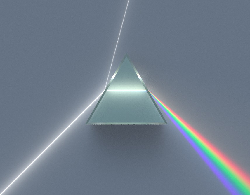
The refractive index of most materials varies with the wavelength of light. In other words, the velocity of light in a crystal varies with the light’s color. This variation is dispersion. One consequence of dispersion is that different colors of light follow different paths through a crystal because they refract at different angles (according to Snell’s Law). We can sometimes see dispersion in thin sections but it is only readily apparent in a few minerals. An excellent but nonmineralogical example of dispersion is the separation of white light into different colors when refracted by a glass prism (Figure 5.13). When a beam of white light enters and exits a prism, different wavelengths (colors) exit at different angles, resulting in the production of colorful rainbows. Note also the reflected beam of white light in Figure 5.13. Reflection and refraction often occur together; their relative intensities depend on the angle at which the light hits an interface.

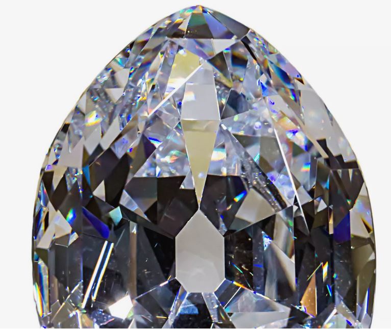
For a mineralogical example of dispersion, we may consider diamond. Diamond’s extreme dispersion accounts, along with its high refractive index, for the play of colors (fire) that diamonds display (seen in Figure 5.14). If not for dispersion, diamonds might sparkle, but the sparkles would all be the same color. Minerals with low dispersion generally appear dull no matter how well cut or faceted. They may, however, be useful as lenses because dispersion can separate colors and cause unwanted effects.

A mineral’s refractive index and dispersion profoundly affect its luster. Minerals with both very high refractive index and dispersion, such as diamond or cuprite, appear to sparkle and are termed adamantine. Minerals with a moderate refractive index, such as spinel and garnet (n = 1.5 -1.8), may appear vitreous (glassy) or shiny; those with a low refractive index, such as borax, will appear drab because they do not reflect or refract as much incident light. Refractive index depends on many things, but a high n-value suggests minerals composed of atoms with high atomic numbers, or of atoms packed closely together.

5.3 Polarization of Light

5.3.1 Polarized Light

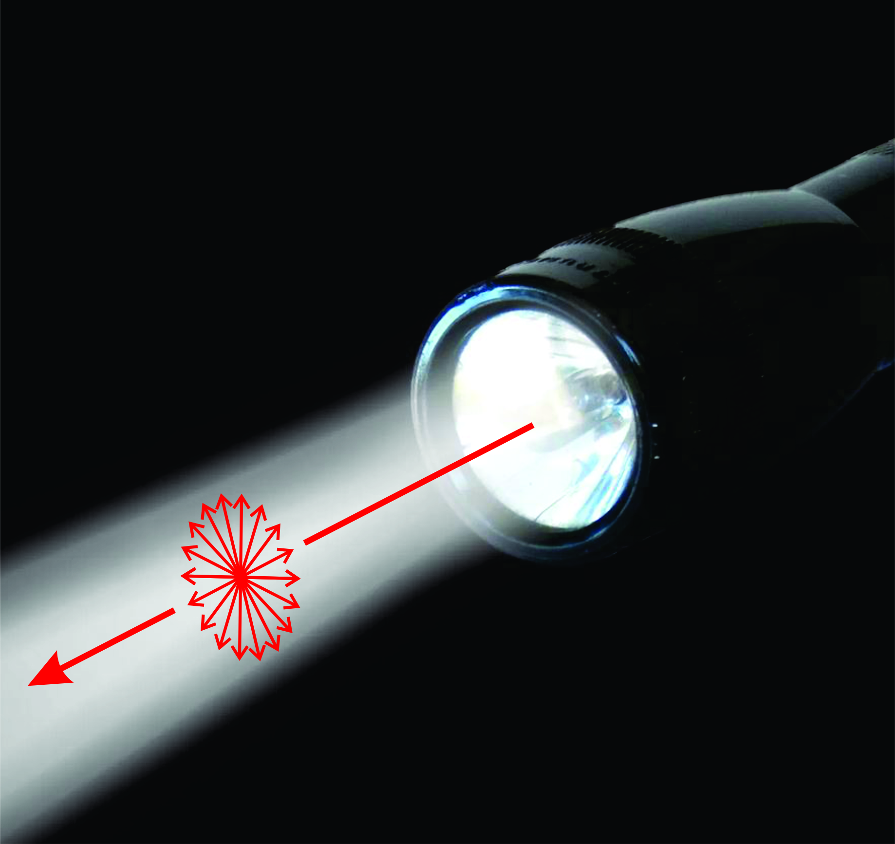
The vibration direction of a light wave (which is the direction of motion of the electric wave) is perpendicular, or nearly perpendicular, to the direction the wave is propagating. In normal unpolarized beams of light, waves vibrate in many different directions, shown by arrows in Figure 5.15.

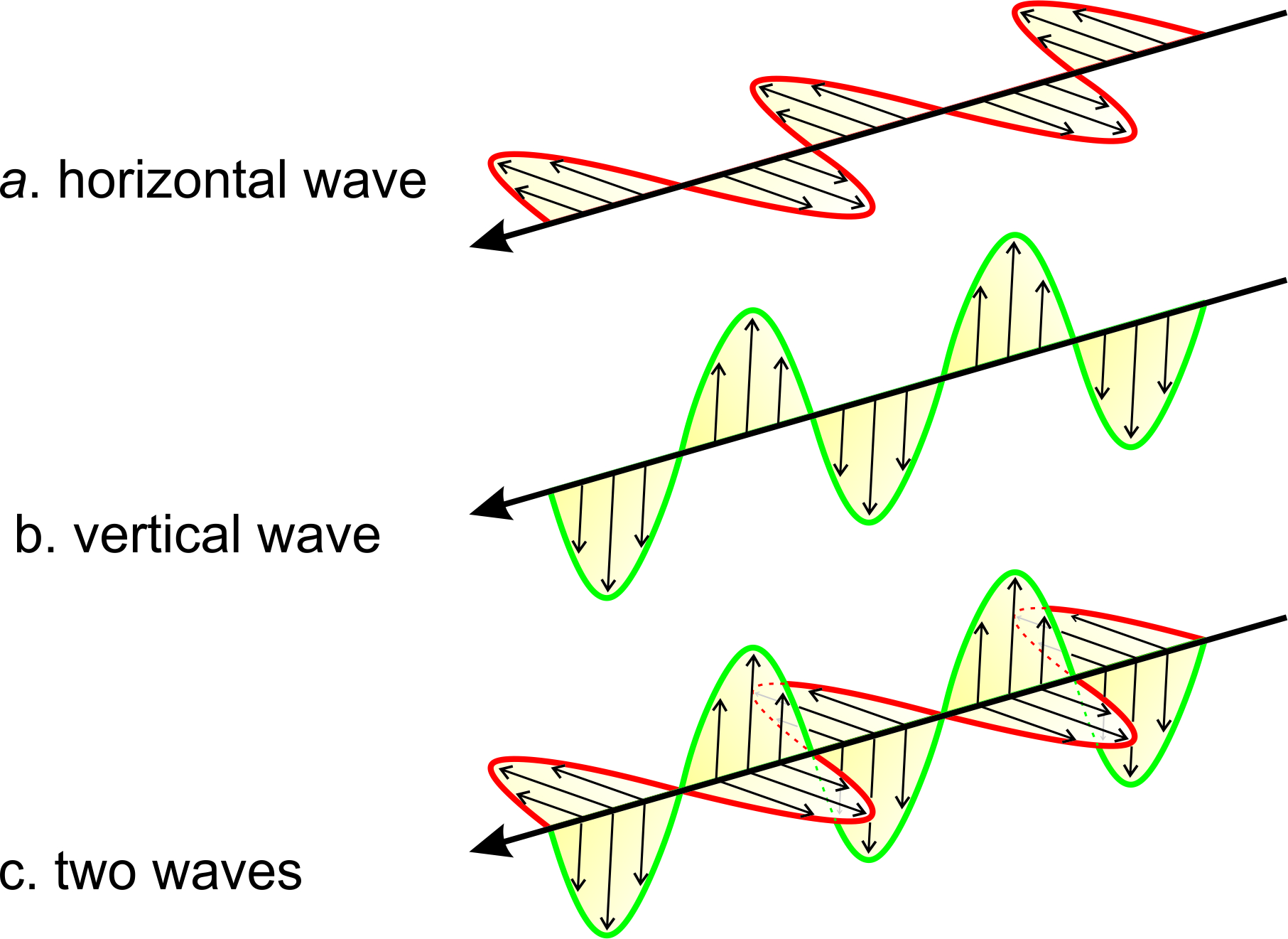
We can filter an unpolarized light beam to make all the waves vibrate in one direction parallel to a particular plane (Figure 5.16). The light is then plane polarized, sometimes called just polarized. (Unlike the drawings in Figure 5.16, a beam of white light, whether polarized or not, may contain many different wavelengths.) Figure 5.16a shows a wave vibrating horizontally and Figure 5.16b shows one vibrating vertically. Figure 5.16c shows the two polarized rays together. They are in phase but need not be.

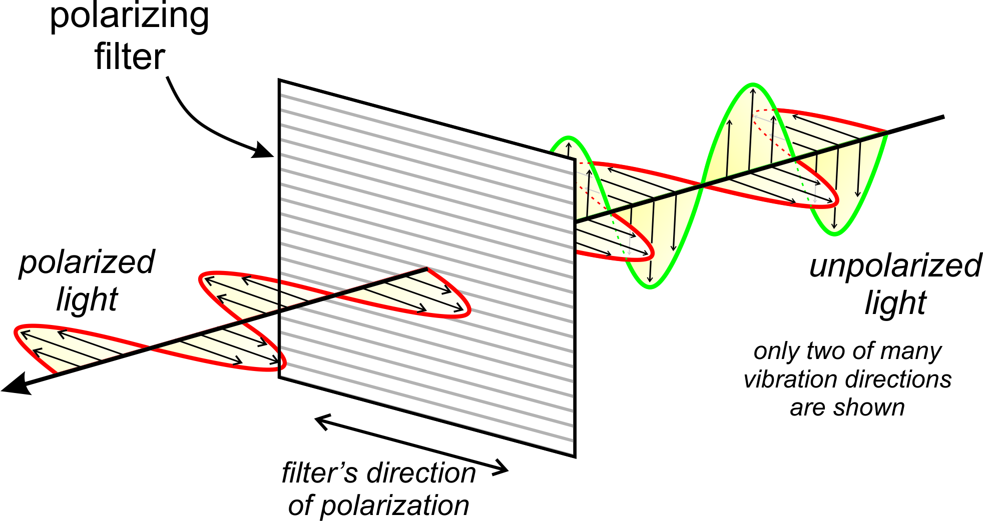
Figure 5.17 shows what happens when a beam of unpolarized light encounter a polarizing filter. Only two vibration directions are shown for the unpolarized light but you should envision light vibrating in all directions before it reaches the filter. After passing through the filter, all light that remains in constrained to vibrate in one plane. It is plane polarized. In this figure, the polarization direction is horizontal, but it could be in any direction if we rotated the filter.

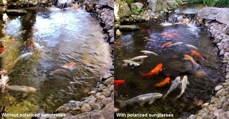
Light becomes polarized in different ways. Reflection from a shiny surface can partially or completely polarize light. Light vibrating in planes parallel to the reflecting surface is especially well reflected, while light vibrating in other directions is absorbed. This is why sunglasses with polarizing lenses help eliminate glare. Figure 5.18 contains two views of a stream containing fish. The view on the left shows lots of glare caused by light reflecting from the water surface. The light is polarized horizontally because the surface is horizontal. The view on the right is through a polarizing filter that only allows us to see light vibrating vertically. Reflections from roads and many other surface cause glare that can be eliminated with polarizing sunglasses.

5.3.2 Crossed Polars

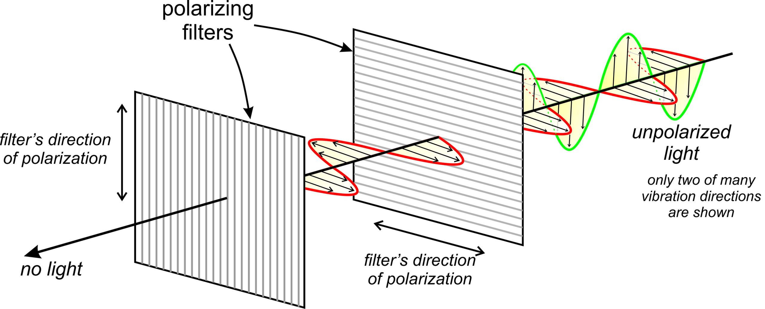
Suppose light passes through a polarizing filter that constrains it to vibrate horizontally (Figure 5.19). (In this figure, we only show two of the many vibration directions in the unpolarized light but think of vibrations occurring in all directions.) On the other side of the first filter, the polarized beam, although perhaps decreased in intensity, appears the same to our eyes because human eyes cannot determine whether light is polarized. If, however, a second polarizing filter, oriented perpendicularly to the first filter, is in the path of the beam, we can easily determine that the beam is polarized. If the second filter allows only light vibrating in a north-south direction to pass, no light will pass through it.

Figure 5.20 shows some polarizing filters piled randomly on top of each other. In some places the filters are at 90^o to each other and no light gets through. In other places they transmit lots of light. (These filters have a gray color and absorb some light, so we do not see any white light being transmitted no matter the orientation of the filters.) But, when the filters are aligned we get maximum light transmission, and when they are perpendicular we get none.

5.3.3 Polarized Light Vibrating at an Angle to a Polarizing Filter

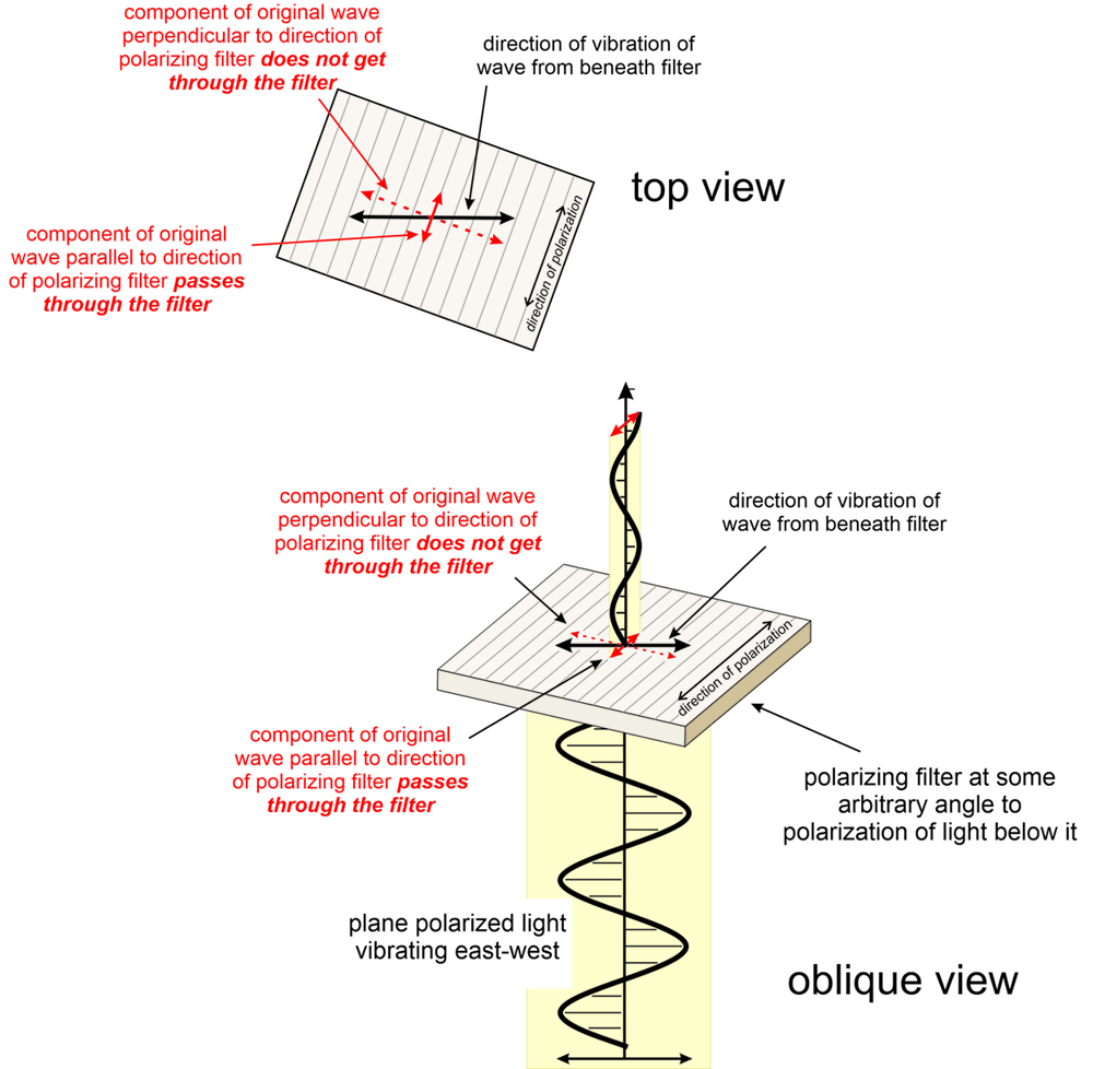
Suppose polarized light hits a polarizing filter at some angle such that the light is vibrating neither parallel, nor perpendicular, to the polarization direction of the filter. In this case, only the component of the light that is vibrating parallel to the filter will pass. The filter absorbs the rest.

Figure 5.21 shows this happening. An original light beam travels vertically from below and encounters a filter. The light is vibrating nearly perpendicularly to the vibration direction of the filter but a small amount – the component that is vibrating parallel to the filter – gets through. If we rotated the filter, the amount of light transmitted would range from 0 to 100% depending on the orientation of the filter with respect to the polarization direction of the light from below. If the light from below is polarized east-west and the filter is polarized north-south, no light will pass through it (Figure 5.19). If we slowly rotate the filter to an east-west orientation, it will gradually transmit more light, and eventually, all of the light.

5.4 Petrographic Microscopes

5.4.1 The Components of a Microscope

Polarizing microscopes, like the one seen in Figure 5.22, are in many respects the same as other microscopes. They magnify small features in a thin section so we can see fine details. These microscopes include many components. We view thin sections in two modes, depicted in Figure 5.23.

Orthoscopic illumination is standard and by far the most commonly used method. It involves an unfocused light beam that travels from the substage, through the thin section, and straight up the microscope tube to the ocular lens and our eyes. The light rays travel perpendicular to the stage and perpendicular to a thin section on the stage.

 

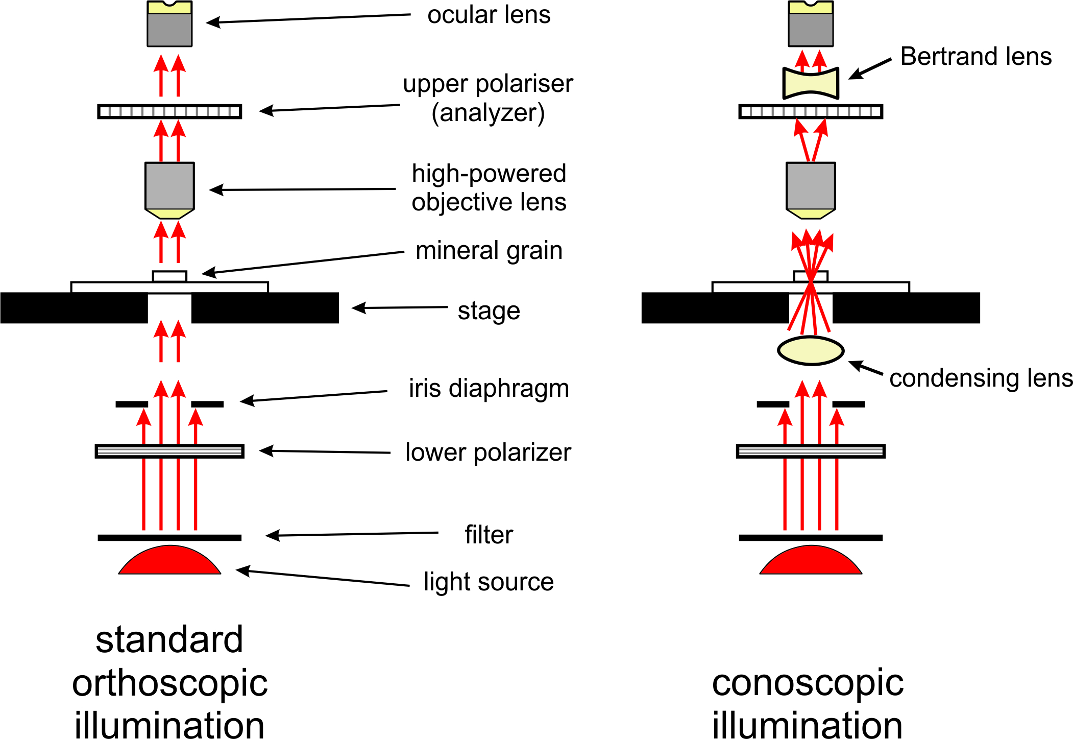
For some purposes, we insert a special lens called, a conoscopic lens, between the lower polarizer and stage to produce conoscopic illumination (also shown in Figure 5.23). The conoscopic lens, also called a condenser lens, causes the light beam to converge (focus) on a small spot on the sample. So, light illuminates the sample with a cone of nonparallel rays. The light then travels up the microscope tube in many directions instead of only vertically. Above the upper polarizer, most microscopes have a Bertrand lens that causes light to again travel vertically before it reaches the ocular.

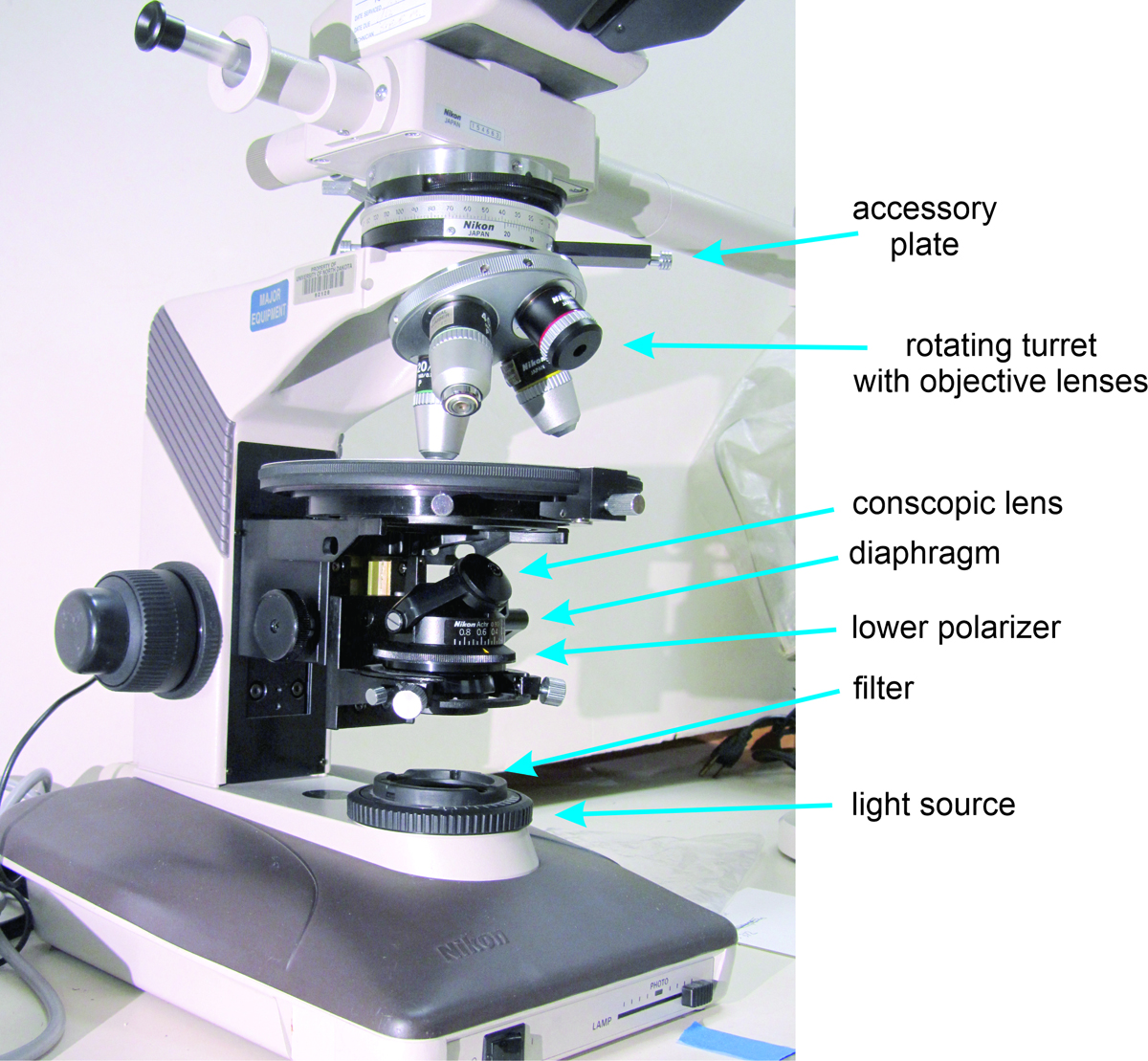
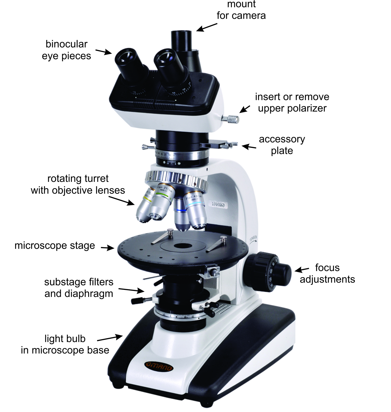
Figures 5.22 and 5.24 show the most important microscope components. A bulb beneath the microscope stage provides a white light source. The light passes through several filters, the lower polarizer, and a diaphragm that can limit the size of the light beam. When polarized white light reaches the stage, it interacts with the material being observed. Ultimately, the light reaches our eye(s) and we see the sample.

The most important filter below the stage is the lower (substage) polarizer, which ensures that all light striking the sample is plane polarized (vibrating, or having wave motion, in only one plane). The presence of a substage polarizer sets petrographic/polarizing microscopes apart from other microscopes. In most modern polarizing microscopes, the lower polarizer only allows light vibrating in an east-west direction to reach the stage. Older microscopes, however, may have the lower polarizer oriented in a north-south direction. Above the polarizing filter, a diaphragm helps concentrate light on the sample.

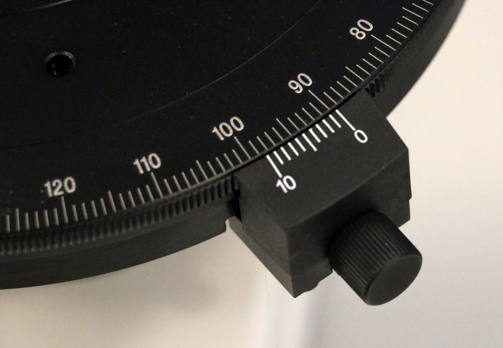
Because most minerals are anisotropic, the interaction of the light with a mineral varies with stage rotation. We can rotate the microscope stage to change the orientation of the sample relative to the polarized light. A calibrated angular scale around the outside of the stage allows us to make precise measurements of crystal orientation (Figure 5.25). The scale is also useful for measuring angles between cleavages, crystal faces, and twin orientations, and for measuring other optical properties.

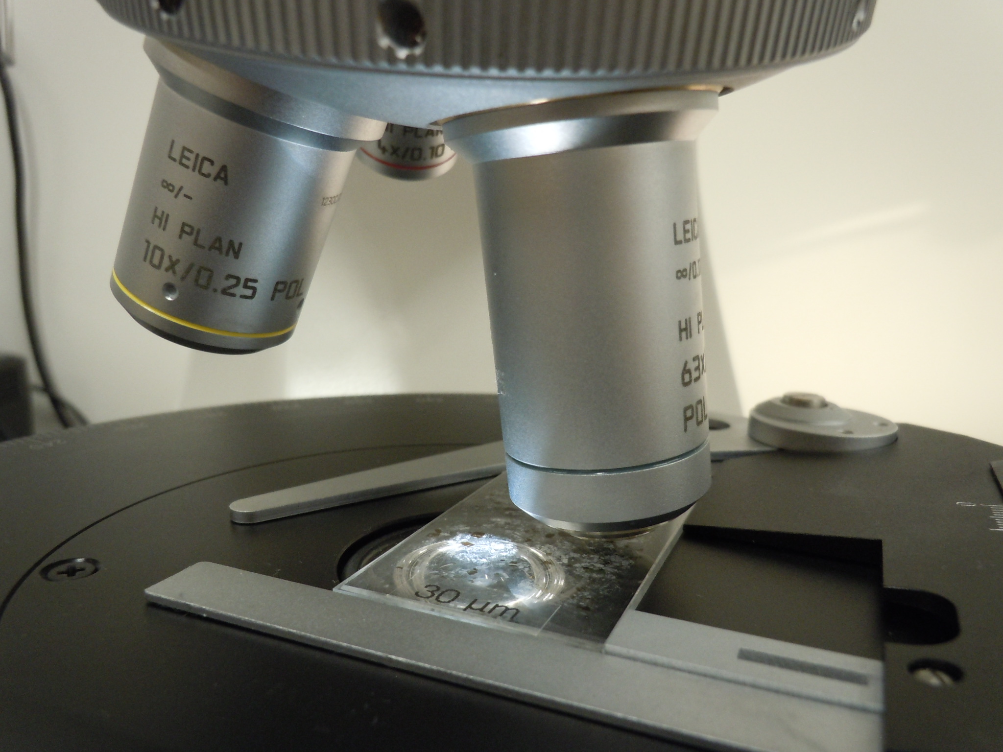
A rotating turret above the microscope stage holds several objective lenses (Figure 5.26). Typically, they range in magnification from 4x to 64x. Different objective lenses can have different numerical apertures (NA), a value that describes the angles at which light can enter a lens, which is an important consideration when making some kinds of measurements. In the discussion of interference figures later in this chapter, we have assumed that the objective lens being used has an NA of 0.85, since this is by far the most common today. (For lenses with a different NA, some angular values in the discussion of interference figures later in this chapter will be in error.)

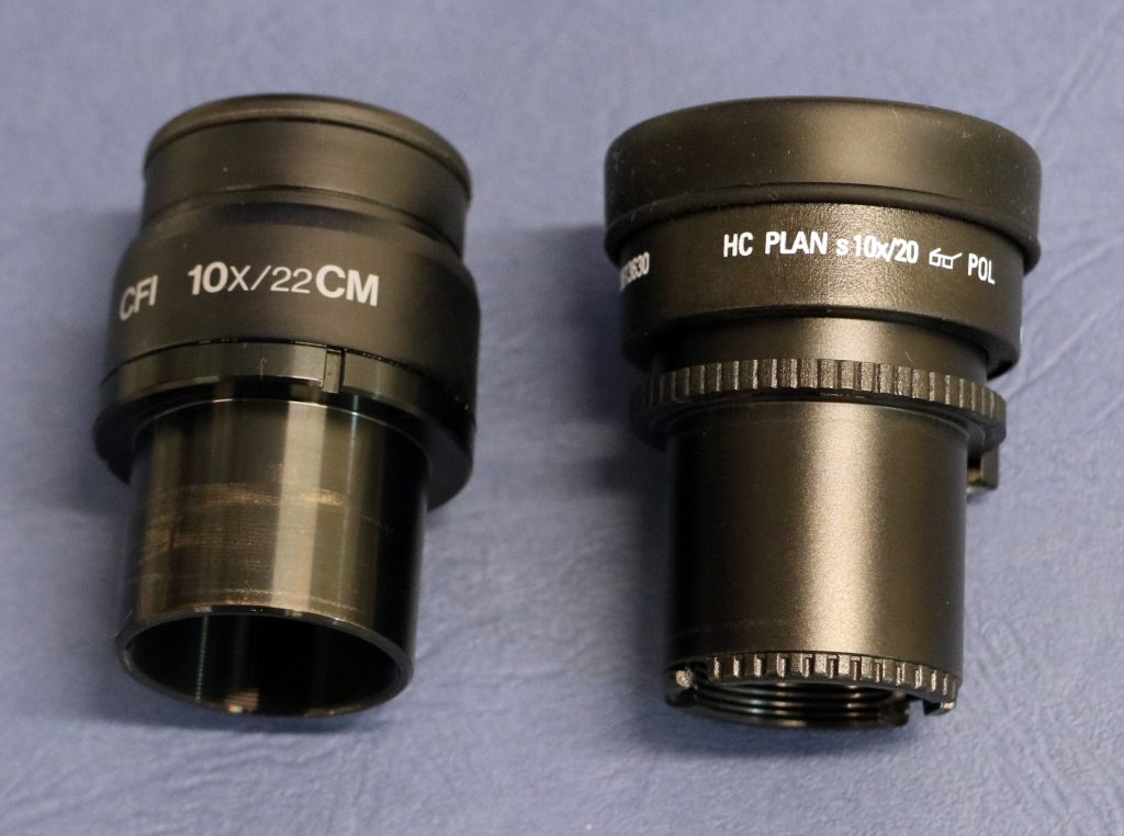
Microscope eyepieces contain additional lenses, called oculars, usually providing 8x or 10x magnification. (The eyepieces shown in Figure 5.27 have 10x magnification written on them.) Older microscopes only had one eyepiece but today most are binocular microscopes with two eyepieces and two oculars. Oculars have crosshairs that aid in making measurements when we rotate the stage. The total magnification, which is the product of the objective lens magnification and the ocular magnification, varies from about 16x to 500x, depending on the lenses used.

Petrographic microscopes have other filters and lenses between the objective lens and the ocular (shown and labeled in Figures 5.22, 5.23, and 5.24). The upper polarizer, sometimes called the analyzer, is a polarizing filter oriented at 90° to the lower polarizer. We can insert or remove it from the path of the light beam. If no sample is on the stage, light that passes through the lower polarizer cannot pass through the upper polarizer. If a sample is on the stage, it usually changes the polarization of the light so that some can pass through the upper polarizer.

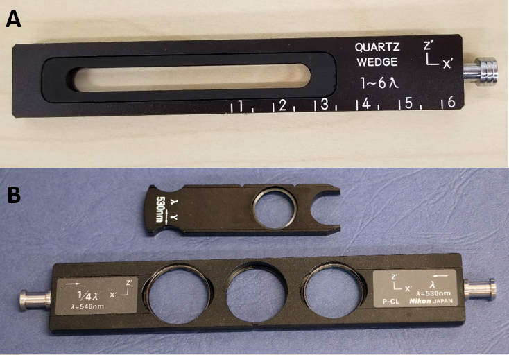
We can also insert a quartz wedge or an accessory plate below the upper polarizer. (A quartz wedge is exactly what it sounds like – a sliver of quartz that is thicker at one end than at the other.) The most common kind of accessory plate used today is a full wave plate. In the past, all full-wave plates were made of gypsum but today they are made of quartz. A wedge or an accessory plate modify light properties for making some specific kinds of observations.

 

5.4.2 Plane (PP) Polarized Light and Cross Polarized (XP)Light

For routine viewing, petrologists and mineralogists use polarizing microscopes with orthoscopic illumination, and with, or without, the upper polarizer inserted. Without the upper polarizer, we see a sample in plane-polarized light, also called PP light. With the upper polarizer, we see it in cross-polarized light, also called crossed polars or XP light. Grain size, shape, color, cleavage, and other physical properties are best revealed in PP light. The optical properties refractive index and pleochroism are also determined using PP light. We use XP light, sometimes focused with conoscopic and Bertrand lenses, to determine other properties including retardation, optic sign, and 2V. To see examples of all of these properties and many views of the most common minerals in thin section go to our Optical Mineralogy website.

We will discuss mineral properties in XP light later in this chapter. For now, we will concentrate on plane polarized light.

5.4.2.1 Characteristics Seen in Plane Polarized (PP) Light

•Opaque and Nonopague Minerals

Opaque minerals, in contrast with nonopaque minerals, do not allow any light to pass through them. So, opaque grains appear black in both PP and XP light, even if we rotate the stage. The most common opaque minerals include graphite, oxides such as magnetite or ilmenite, and sulfides such as pyrite or pyrrhotite. It is sometimes possible (especially if a thin section does not have a cover slip) to remove a slide from the microscope stage, hold it up and turn it around, and reflect light off mineral grains to see the reflected color. A silver color suggests the grains are graphite or oxides and a golden color suggests they are sulfides.

•Crystal Shape and Habit

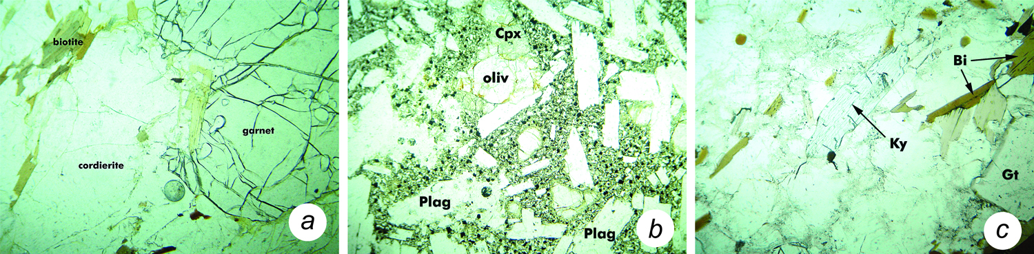
When viewing minerals in PP light, we can pick out different minerals based on their grain shapes and habit. For example, Figure 5.29a below shows a large rounded grain of garnet containing many sharp fractures. Figure 5.29b contains lathes of clear plagioclase (Plag), an equant grain of olivine (oliv) and an almost rectangular grain of clinopyroxene (Cpx). Figure 5.29c has a large blade of light blue kyanite in the center of the view. Both Figures 5.29a and c contain flakes of brownish biotite (Bi).

•Cleavage

The garnet, cordierite, and olivine seen in Figure 5.29 show no cleavages (although the garnet does display many fractures). Many minerals, however, exhibit cleavage, usually appearing as straight parallel cracks through a grain. When we can see cleavage with a microscope, it can be an important diagnostic tool. We use qualitative terms such as perfect, good, fair, and poor (discussed in Section 3.5.2, Chapter 3) to describe the ease with which a mineral cleaves in different directions. Minerals with one or more good or perfect cleavages show cleavage most of the time, while those with only poor cleavage may not. Additionally, minerals with low relief do not show cleavage as readily as those with high relief. We can overcome this problem sometimes by closing down the substage diaphragm, which narrows the cone of light hitting the thin section and increases contrast.

Minerals may have zero, one, two, three, four, or even more cleavages, but because thin sections provide a view of only one plane through a mineral grain, we rarely see more than three at a time. And minerals that have elongate habits exhibit different cleavage patterns when viewed in a cross section than they do when viewed in a longitudinal section.

When we look at a mineral grain in thin section we are looking in a singular direction through the mineral. But cleavage planes are oriented in three dimensions (3D). So observed cleavage angles depend on grain orientation. If a mineral has two cleavages that intersect at 60°, the cleavages will appear to intersect at any angle from 0° to 60° depending on grain orientation. So we must often examine many grains (or one with a known orientation determined by examining an interference figure) to learn the maximum, and true, 3D cleavage angle.

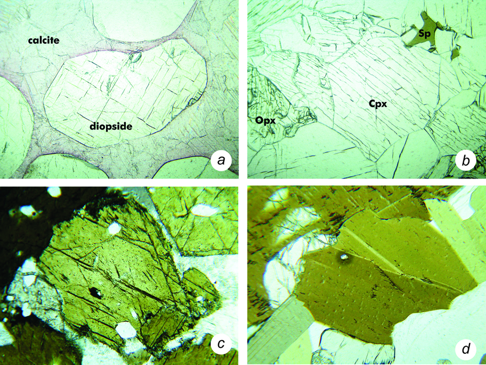
Figure 5.30a shows a grain of diopside with two perpendicular cleavages. Figure 5.30b shows augite, a pyroxene closely related to diopside, but the grain is at a different orientation and shows only one direction of cleavage. Figure 5.30c shows a brown amphibole grain with two cleavages that intersect at about 60° and 120°. If the grain were oriented differently, only one cleavage might be visible. Figure 5.30d shows several grains of biotite. The tilted greenish rectangular grain near the lower left corner shows good mica cleavage (cleavage in one direction). The large darker brownish grain that fills most of the view does not because the view is looking down on top of a flake.

•Color and Pleochroism

When we talk about the color of a mineral in thin section, we are talking about its color when viewed with PP light, not when viewed with XP light. Many minerals appear colored in hand specimen, and some show color when viewed with a microscope. But it is rare for the reflected color of a hand specimen to have any resemblance to the transmitted color seen in thin section.

The difference is due to several things. Most importantly, when we see color in a hand sample, we are seeing the color of light reflected by the sample. If all colors reflect, the sample appears white. If none reflect, it is black. And if only some wavelengths reflect we see various colors. This is not what happens when we view minerals in thin section.

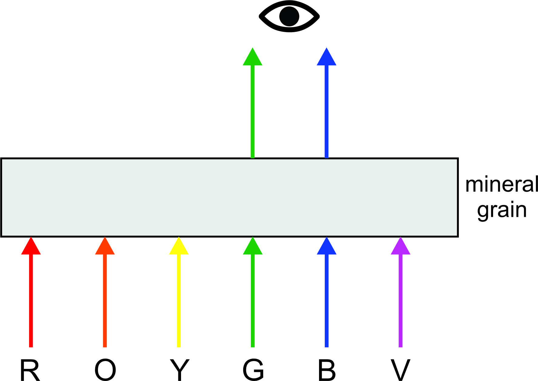
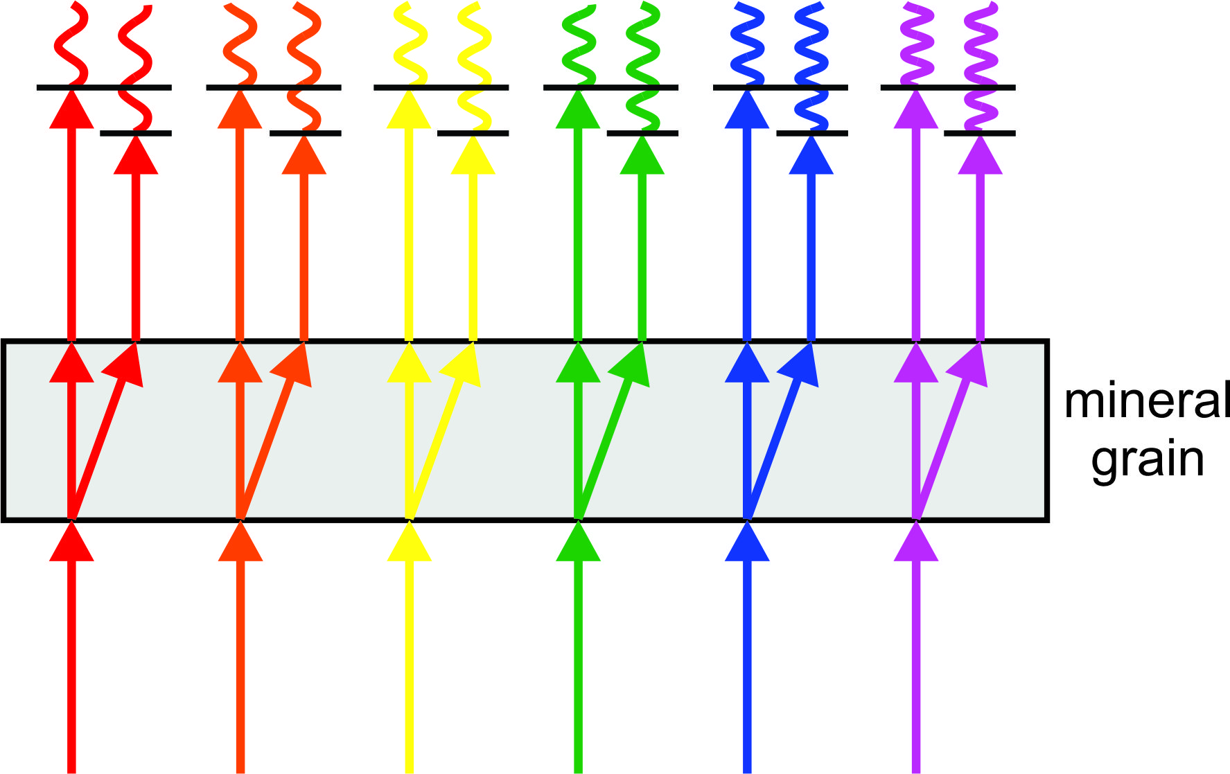
When we see color in thin section (using PP light) we are seeing transmitted colors. These are the colors of light passing through a mineral grain (Figure 5.31). Crystals absorb some wavelengths and transmit others. If all colors are transmitted, we see white. If none are transmitted, we see black. And in other cases we see colors of different hues depending on the mineral’s absorption. But many minerals in thin section are not thick enough to significantly absorb specific wavelengths of light. So minerals in thin section often appear light colored even if the mineral has strong coloration in hand specimen.

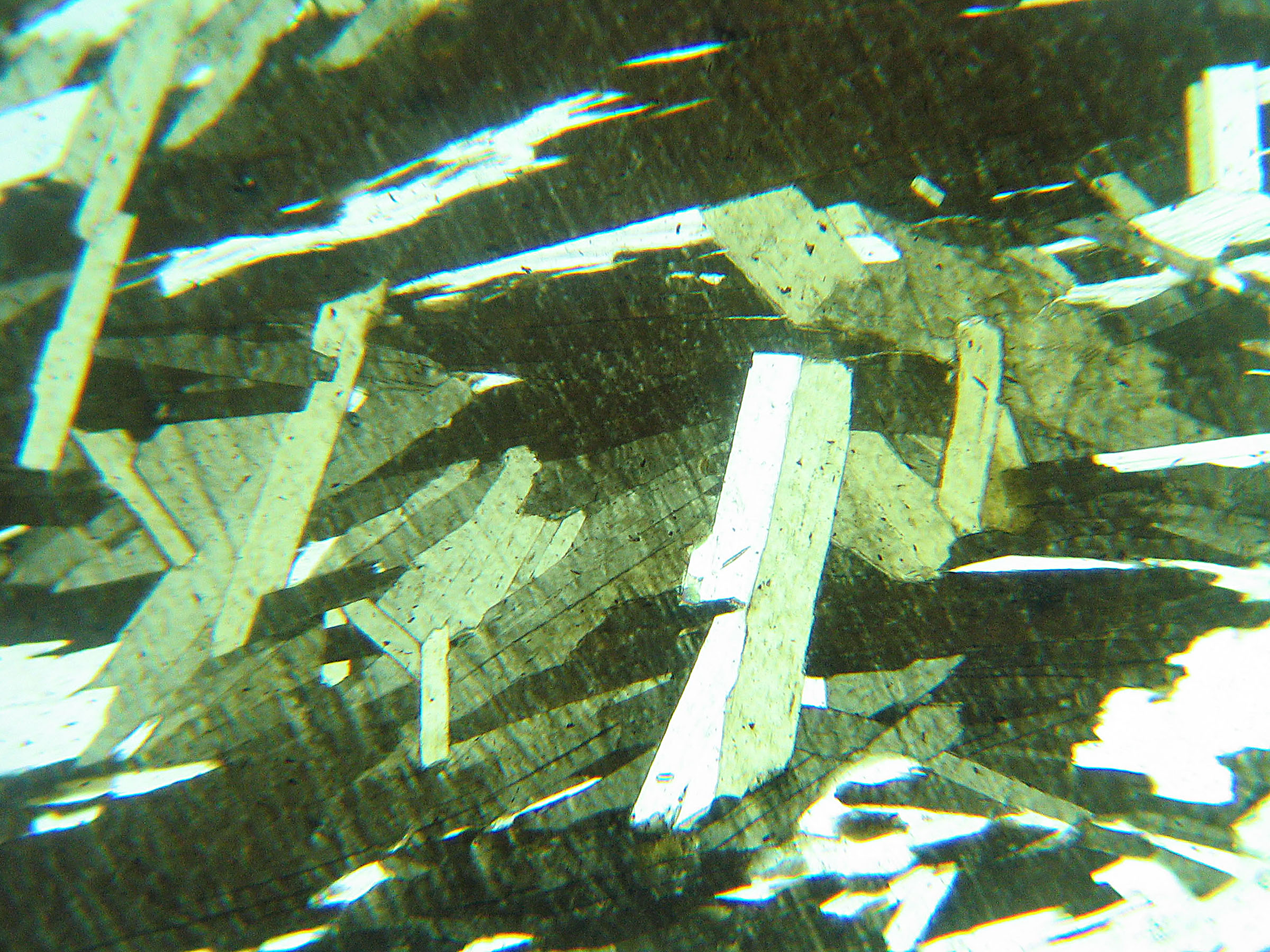
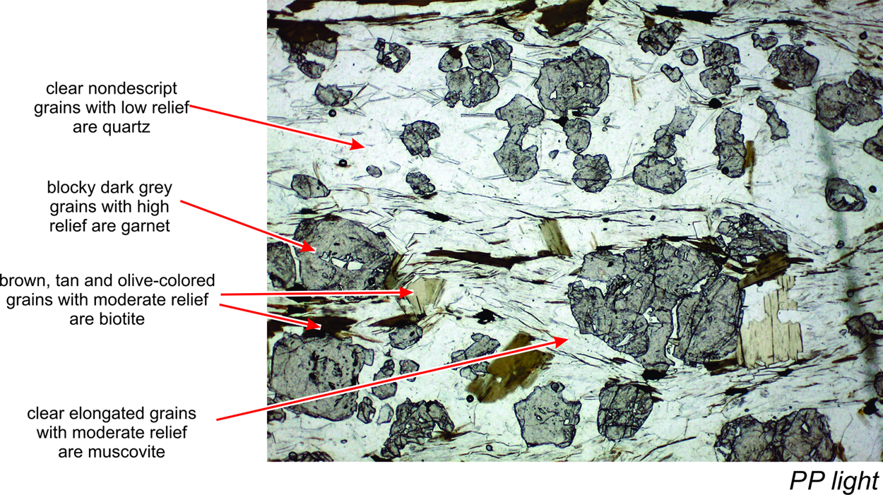
Figure 5.32 shows a mica schist, viewed with PP light. The minerals present include biotite in various shades of greenish brown and tan, clear elongated clear crystals of muscovite and somewhat equant quartz (on the lower right edge). Biotite is generally black when viewed in hand specimen but always is lighter colored in thin section, like the biotite seen here. Different grains of biotite have different colors because they have different atomic orientations with respect to the light vibration direction. In this thin section, the few grains of muscovite (white mica) have the same shape as the biotite (because they are both micas) but show no coloration.

Many minerals absorb different wavelengths of light depending on light vibration direction. So colors we see in thin section generally change when we rotate the microscope stage. This is because rotating the stage changes the orientation of the mineral’s crystal structure with respect to the polarized light passing through the lower polarizer. We call this property (changing colors with stage rotation) pleochroism. Biotite is an example of a mineral that normally displays marked pleochroism. If we rotated the sample seen in Figure 5.32, biotite colors would vary between various shades of brown or tan. The exact colors depend on the biotite composition. For a typical grain, color varies between two hues. The range of color, however, depends on grain orientation in the thin section.

▶️  Video 2: Explanation of color and pleochroism (3 minutes)

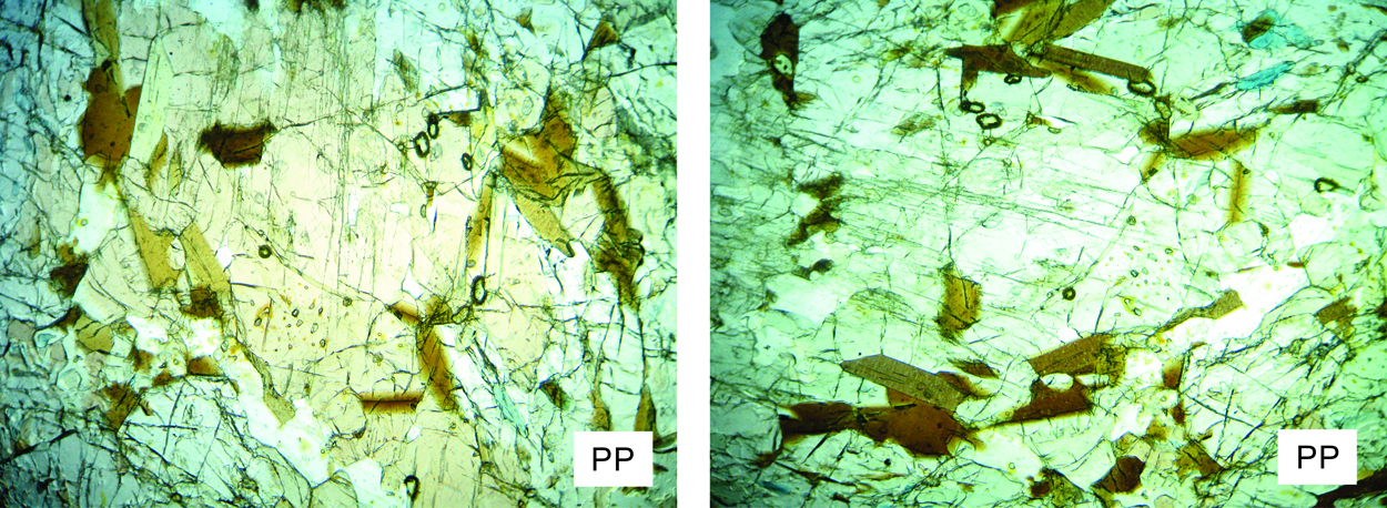
Pleochroism is an especially useful diagnostic property when identifying some minerals, but it can be overlooked because it may be subtle. For example orthopyroxenes are nearly colorless in thin section, but some show a faint pleochroism from (what mineralogists call) pink to green. The photos in Figure 5.33 show the same large grain of orthopyroxene but the orientation of the grain is 90^o different in the two views. Light pinkish color can be seen in the photo on the left, and light green color in the photo on the right. Pleochroism of pyroxenes is an important property because it sometimes distinguishes the two major pyroxene subgroups: orthopyroxenes and clinopyroxenes.

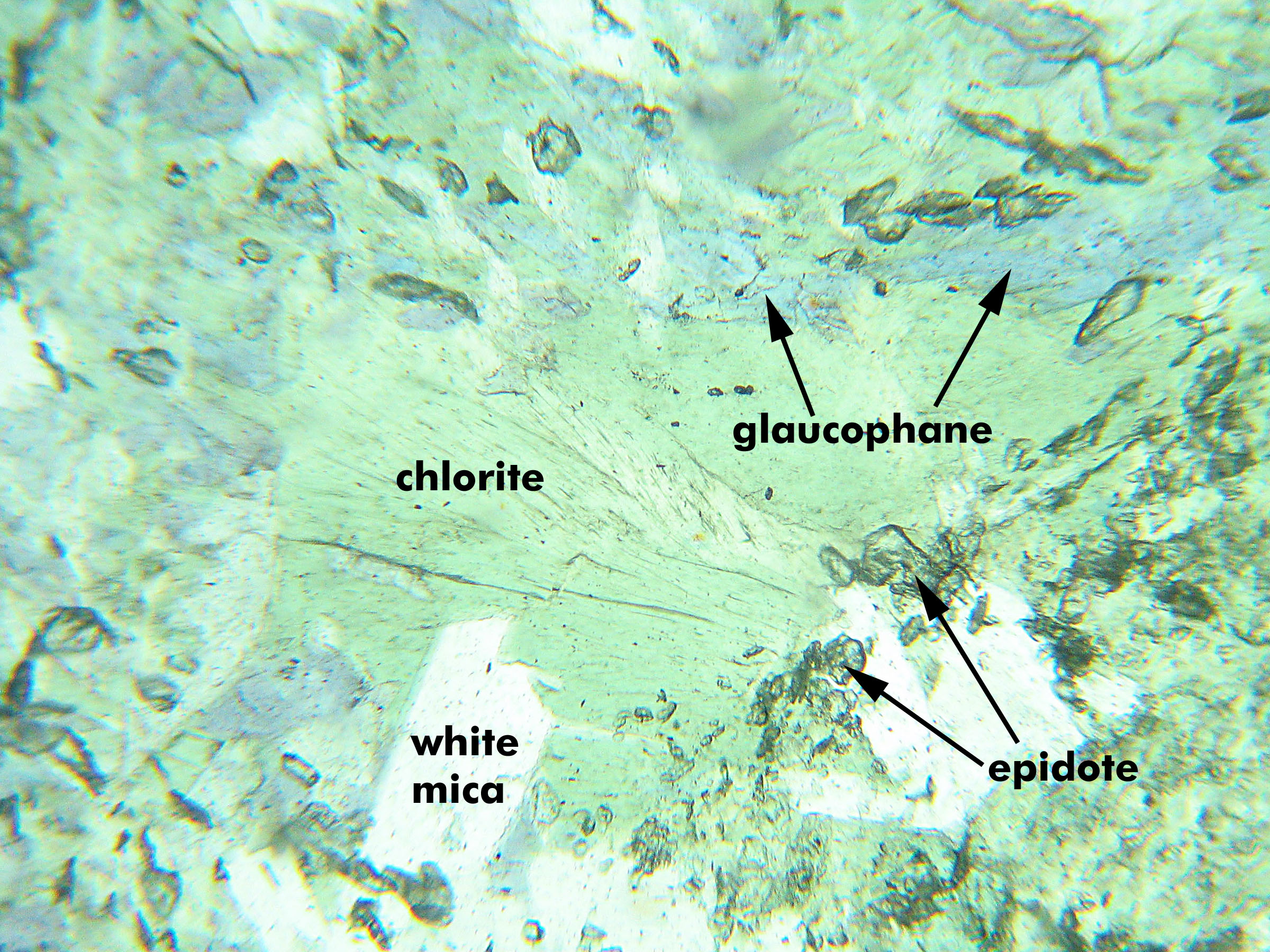
In contrast with orthopyroxenes, many amphiboles display strong colors and a very noticeable pleochroism in thin section. For minerals, such as amphiboles, that have noticeable pleochroism, reference tables give pleochroic formulas that describe the colors seen when looking at grains in different directions through the crystal’s atoms. The hornblende in Figure 5.4, for example, is pleochroic in various shades of green. And the biaxial mineral glaucophane (an amphibole shown in Figure 5.34) has pleochroism described by the pleochroic formula:
blank• X = colorless or pale blue
blank• Y = lavender-blue or bluish green
blank• Z = blue, greenish blue, or violet

X, Y, and Z refer to light vibrating parallel to each of three mutually perpendicular vibration directions in a crystal. In thin sections, glaucophane’s colors vary within the limits described for X, Y, and Z, depending on the crystal orientation, as we rotate the microscope stage. Figure 5.34 shows blue glaucophane in a rock from Panoche Pass, California. Different grains of glaucophane show different hues due to different grain orientations. Figure 6.88 (Chapter 6) shows a hand sample of glaucophane; it is one of a small number of minerals that have colors in thin section that are quite similar to those seen in hand sample.

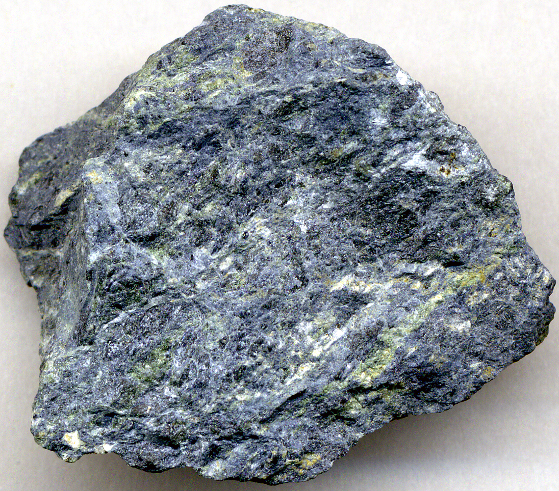
For another example of pleochroism, consider the biotite in Figure 5.32. It is pleochroic in browns, and a standard pleochroic formula for biotite might be:
blank• X = colorless, light tan, pale greenish brown, or pale green
blank• Y ≈ Z = brown, olive brown, dark green, or dark red-brown

•Relief and Becke Lines

If epoxy or some other material with significantly different refractive index surrounds mineral grains, the grains will stand out. This is the case for the garnet in epoxy in Figure 5.35A. But, if mineral grains are surrounded by material that has a similar refractive index to the mineral, they may be almost invisible unless the mineral is one of the few minerals with very strong coloration. This is the case for the halite grains seen in a grain mount in Figure 5.35B. As the difference between the index of the surrounding material and the mineral decreases, the boundary between the two becomes less easily distinguished. The term relief describes the contrast between the mineral and its surroundings.

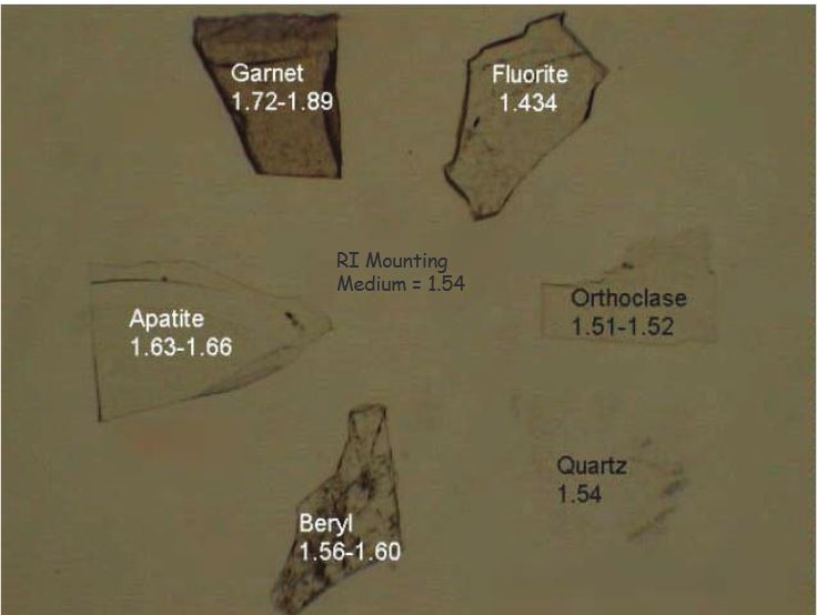
In grain mounts, we often look at mineral fragments surrounded by immersion oil with a specific refractive index. Figure 5.36 shows how relief changes depending on the difference between refractive index of a mineral and surrounding oil. The oil has refractive index of 1.54, but the minerals mostly do not. The garnet and fluorite both have high relief. The other minerals have variable relief, and the quartz almost disappears because quartz and the surrounding oil have the same refractive index.

 

Grains mounts show relief well, but minerals in thin sections also show relief. The relief depends on the difference in the indices of refraction of the mineral and the material (today usually a special type of epoxy) in which it is mounted. Thin section epoxy typically has an index of refraction of 1.54-1.56. As the difference in indices increases, relief becomes more noticeable. We can see relief with either a monocular or a binocular microscope, but more easily with the latter. Some, not all, people see relief in three dimensions when viewing a thin section with a binocular microscope.

Minerals with high refractive indices show high positive relief because their index of refraction is greater than that of the epoxy. They also show structural flaws, such as scratches, cracks, or pits, more than those with low refractive indices. The thin section in Figure 5.37 contains very high relief garnet, moderate relief biotite and muscovite, and low relief quartz. A few minerals (such as calcite) display variable relief with stage rotation; variable relief is a useful diagnostic property for calcite.

Most minerals that appear to have high relief have high refractive indices. But some minerals (fluorite, for example) with very low refractive indices show high relief (termed negative relief) in thin section because their index of refraction is much lower than that of the epoxy. We do not differentiate between positive and negative relief in this book; for most purposes, we need only to know whether a mineral displays high, medium, or low relief – which really means whether it stands out in thin section.

When we immerse a mineral grain in liquid that has refractive index different from the mineral’s, refraction occurs and some light rays bend toward the medium with the higher refractive index. Other light rays are completely reflected because they hit the mineral-liquid interface at an angle greater than the critical angle of refraction. But overall, light interacts with a mineral grain as if the grain were a small lens (Figure 5.38).

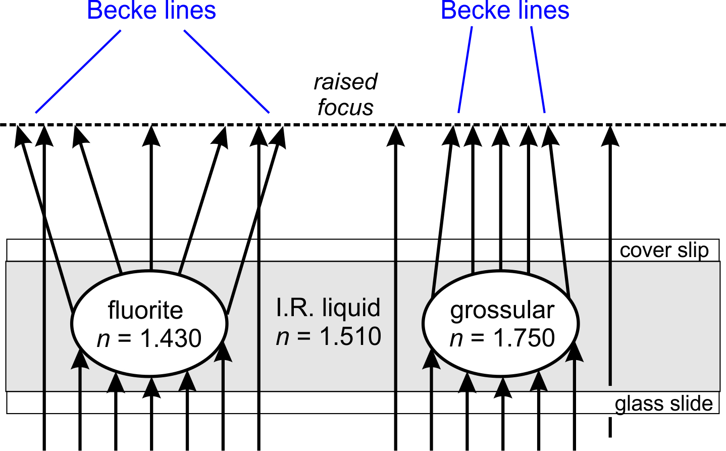
If n_mineral < n_liquid, light rays are refracted and diverge after passing through the grain. If n_mineral > n_liquid, light rays are refracted and converge after passing through the grain. If we slowly lower the microscope stage, shifting the focus to a point above the mineral grain, a bright narrow band of light called a Becke line appears at the interface and moves toward the material with higher refractive index. A complementary but more difficult to see dark band moves toward the material with lower refractive index.

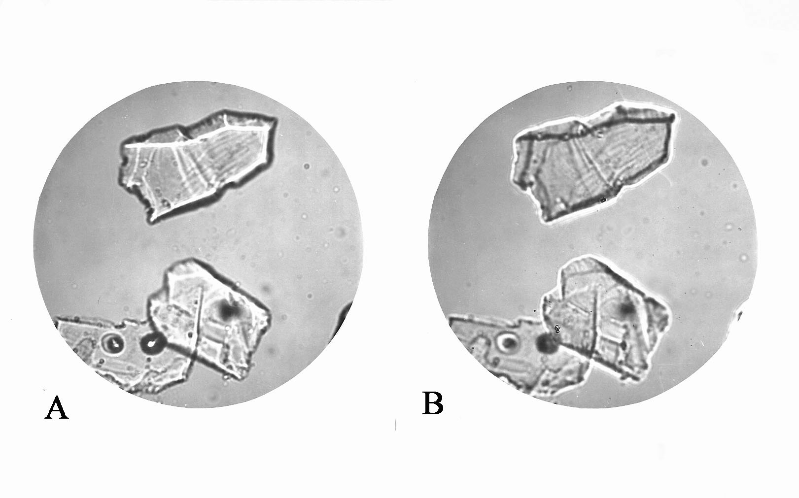
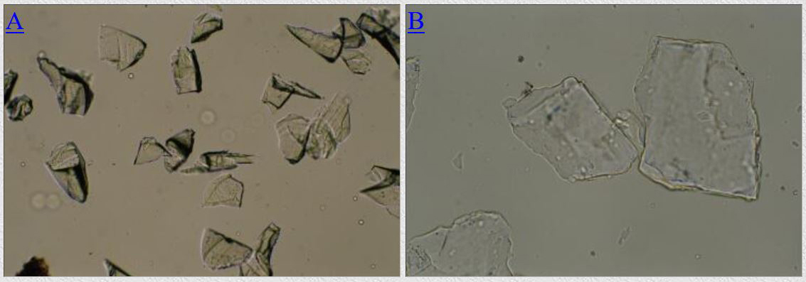
Figure 5.39 shows fragments of a mineral in a refractive index oil significantly different from the mineral. In Figure 5.39A, the microscope focus has been raised (the stage has been lowered), and a white line moved into mineral grains that have higher refractive index than surrounding oil. In Figure 5.39B, the focus was raised (the stage was lowered) and the white line moved outward into oil that has higher refractive index than the mineral grains.

Although not as straightforward, we can also use Becke lines to compare the relief of minerals in thin sections by purposely focusing and defocusing the microscope while we examine a grain boundary. We also compare relief by noting how well a mineral appears to stand out above another.

▶️ Video 3: a good video about Becke lines (5 minutes)

5.4.2.2 Characteristics Seen in Cross Polarized (XP) Light

•Anisotropic vs Isotropic Minerals

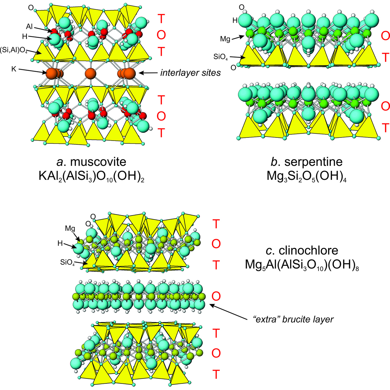
Most minerals are anisotropic. For example, you do not have to look very long at the atomic structures of sheet silicates (Figure 13.30 in Chapter 13) to see that the atom order is different in different directions; they are anisotropic. Because atomic order is not the same in different directions through an anisotropic crystal, refractive index varies with direction. In contrast, a glass, such as window glass or obsidian, is isotropic because it has a random atomic arrangement. Randomness means that, on the average, the structure and refractive index are the same in all directions. Minerals whose crystals belong to the cubic system are isotropic because their atomic arrangement is the same along all crystallographic axes. Minerals belonging to other crystal systems are anisotropic.

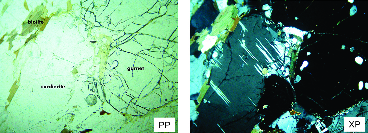
Isotropic minerals are easy to spot in thin sections. When viewed with a polarizing microscope and XP light, they are always extinct, which means they remain black as the stage rotates, no matter what their orientation is on the stage. For example, Figure 5.40 shows PP and XP views of a gneiss containing cordierite and garnet. In the XP view on the right, the garnet is black (isotropic) but the cordierite, which shows stripes due to twinning, is not (anisotropic). There are few common isotropic minerals, but the most common are garnet, sphalerite, and fluorite. Usually we can tell these and the few other isotropic minerals apart by looking at color, relief, habit, and cleavage. Sometimes (poorly made) thin sections contain holes, places with no mineral and only epoxy. The holes appear isotropic and can occasionally be mistaken for isotropic minerals.

In contrast with isotropic minerals, randomly oriented anisotropic mineral crystals do not normally appear extinct when viewed in XP light. But if we rotate the microscope stage, they go extinct briefly every 90°. There is, however, a complication. If an anisotropic crystal is oriented so that light passes through it parallel to a special direction called an optic axis, it will appear to be isotropic. (This occurs when the optic axis is perpendicular to the microscope stage.) In this special orientation the mineral will remain extinct as we rotate the stage.

Fortunately, the number of optic axes in anisotropic minerals is limited to one (in uniaxial minerals) or two (in biaxial minerals). In thin sections, the odds of the optic axis being vertical and parallel to the light beam are small, and confusing isotropic and anisotropic minerals is rarely a problem. When in doubt, we can distinguish them most easily by looking at multiple grains of the same mineral (they cannot all be oriented with their optic axes perpendicular to the stage). We can also distinguish isotropic from anisotropic crystals using conoscopic illumination because anisotropic minerals transmit some conoscopic light and display interference figures (discussed later), while isotropic minerals do not.

•Views Using Crossed Polars

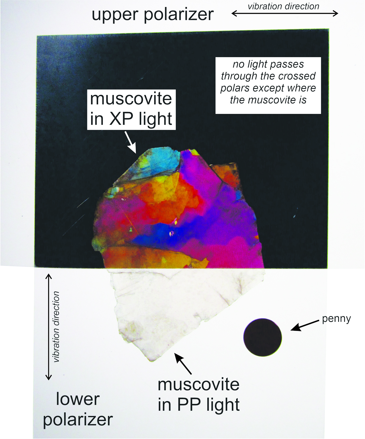
Figure 5.41 shows a ragged flake of muscovite (white mica) with one rectangular polarizing filter below it and another above it. We oriented the filters perpendicularly. So we see black where they overlap and there is no mica. But, where it is present, the mica changes the vibration direction of the light so it can pass through the top polarizer.

Besides changing direction of polarization, when viewed with XP illumination, crystals also change white light to different colors. These are interference colors and, in Figure 5.41, they do not match the color of the mica at all. They appear as various shades of blue, red, orange, and purple. These colors do not result from absorption of different wavelengths by the mineral (which is how minerals get their color when viewed in PP light). Instead, the colors are artifacts of polarized light passing through two polarizers and a crystal. The interference colors in this figure are blotchy and variable because the flaky mica is thicker in some places than in others.

Figure 5.42 shows the origin of the phenomena seen in the previous figure, but with geometry more similar to what happens with a microscope. When no mineral grain is in the path of the light, east-west polarized light encounters a north-south polarizing filter. So, no light is transmitted and only a black color is seen. But, when a flake of mica is present, the grain changes light polarization, so some light gets through the upper polarizer. During this process double refraction occurs (discussed later in this chapter) and the result is interference colors.

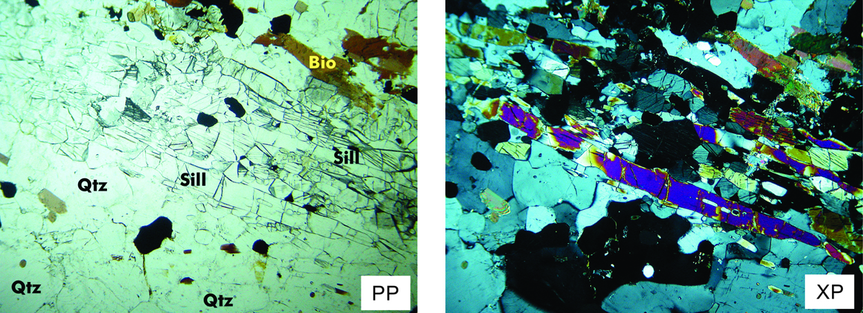
We only see interference colors if we insert the upper polarizer and view a thin section in XP light. For example, the photos in Figure 5.43 show PP and XP views of the same area on a thin section. In the PP view, brown-tan biotite and opaque magnetite (black and unlabeled) are easily seen. But quartz and sillimanite are clear and uncolored.

The XP view in Figure 5.43 is more colorful because it shows interference colors. Interference colors for quartz vary with crystal orientation and would change from white to black if we rotated the microscope stage. Feldspars, and many other minerals have similar white to black interference colors. But most minerals display colors of some sort that may be brighter and more pronounced than colors seen when we view the same mineral in PP light. For example, the long needle of sillimanite in this thin section is clear in PP light. It shows bright purplish-blue colors (that are not completely uniform because the needle is thicker in some places than in other) in XP light. Other grains of sillimanite, which are blocky end-views of needles, show gray or yellow interference colors.

Interference colors are unrelated to the true color of a mineral. And interference colors depend on grain orientation, so different grains of the same mineral in one thin section normally display a range of interference colors. Different minerals display different ranges of interference colors, so color variation is a useful tool for mineral identification. Colors also vary with the thickness of grains, so it is important that thin sections be of uniform thickness. Additionally, the edges of some grains, grains near the edge of a thin section, or grains next to holes in a thin section (places where the sample is thin), may display abnormal interference colors.

•Q. What is the Origin of Interference Colors? A. Double Refraction

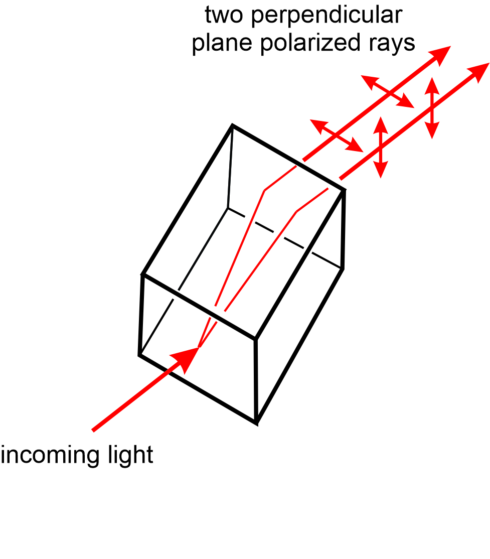
When polarized light encounters an isotropic mineral, it slows as it passes through the mineral, but maintains its character when it emerges. Upon entering an anisotropic crystal, however, light is normally split into two polarized rays, each traveling through the crystal along a different path with a slightly different velocity and refractive index (Figure 5.44). For uniaxial minerals, we call the two rays the ordinary ray (O ray), symbolized by ω, and the extraordinary ray (E ray), symbolized by εʹ. The O ray travels a path predicted by Snell’s Law, while the E ray does not. The directions of the O-ray and E-ray vibrations depend on the direction the light is traveling through the crystal structure, but as seen in Figure 5.44 the vibration directions of the two rays are always perpendicular to each other when they emerge from the crystal.

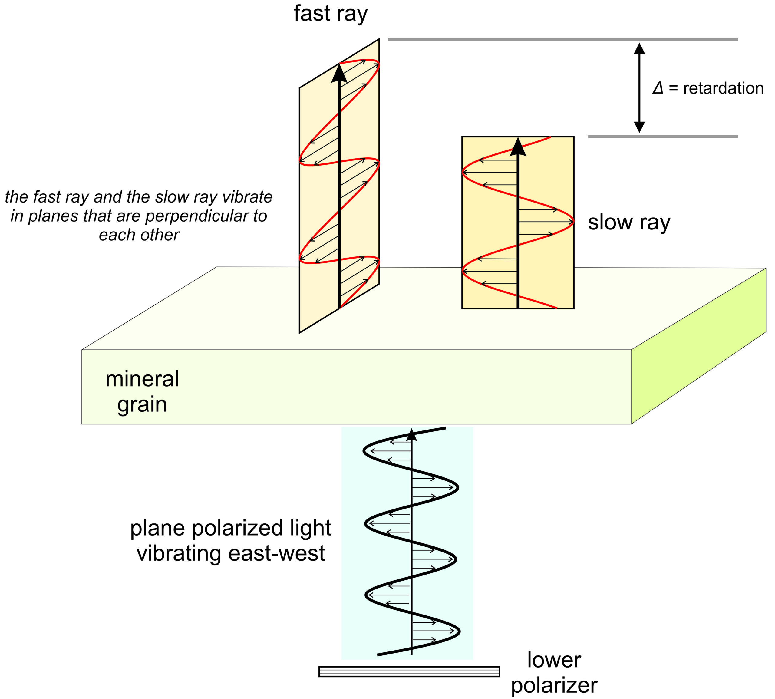
Things are a bit more complicated for biaxial minerals. But, as with uniaxial minerals, a polarized ray encountering a biaxial crystal normally splits into two rays vibrating perpendicularly to each other. One ray emerges from the crystal before the other, so we call the two rays the fast ray and the slow ray. (We also sometimes use the same terms, fast and slow, for the O ray and the E ray of uniaxial minerals, but sometimes the O ray is the fastest and sometimes the E ray is.)

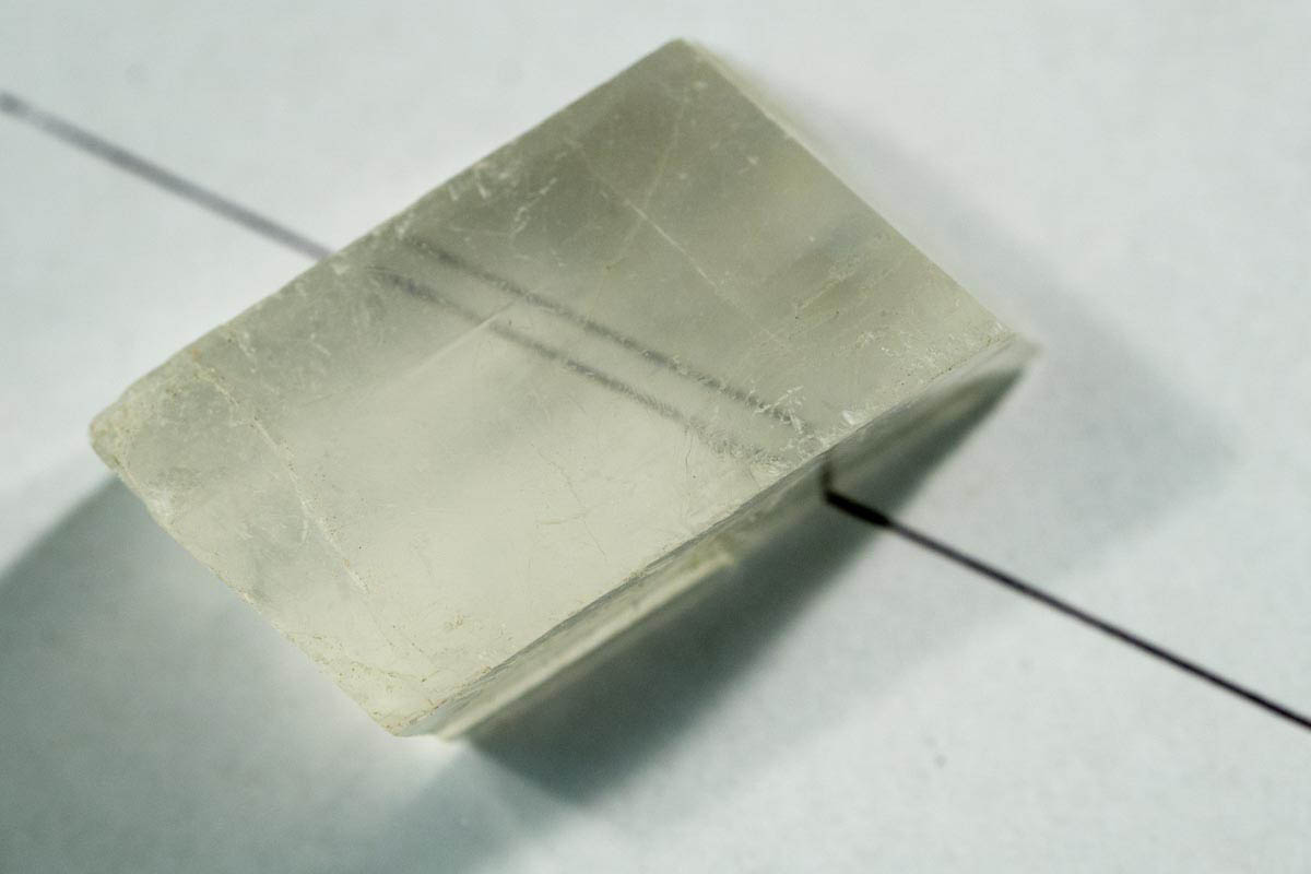
We call the splitting of a light beam into two perpendicularly polarized rays double refraction. All randomly oriented anisotropic minerals cause double refraction. We can easily observe it if we place clear calcite over a piece of paper on which a line, dot, or other image has been drawn (as in Figure 5.45). Two images appear, one corresponding to each of the two rays. A thin piece of polarizing film placed over the calcite crystal would verify that the two rays are polarized and vibrating perpendicular to each other. If we rotate either the film or the crystal, every 90° one ray becomes extinct, and we will see only one image. Calcite is one of a few common minerals that exhibits double refraction easily seen without a microscope, but even minerals that exhibit subtler double refraction can be tested using polarizing filters. Gemologists use this technique to tell gems from imitations made of glass. Glass, like all isotropic substances, does not exhibit double refraction.

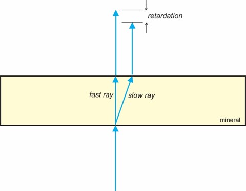
Consider a thin section and light entering an anisotropic mineral grain (Figure 5.46). Double refraction occurs, and as the two rays pass through the crystal (uniaxial or biaxial), they travel at different velocities unless they are traveling parallel to an optic axis. Because the rays travel at different velocities, their refractive indices must be different. The difference in the indices of the fast ray and the slow ray (n_slow – n_fast) is the apparent birefringence (δʹ). It varies depending on the atomic orientation in the crystal and the direction light is traveling. δʹ ranges from zero to some maximum value (δ) controlled by the crystal structure. The maximum birefringence (δ) is a diagnostic property of minerals.

When the slow ray emerges from an anisotropic crystal, the fast ray has already emerged and traveled some distance. This distance is the retardation (Δ), labeled in Figure 5.46. Retardation is proportional to both the thickness (t) of the crystal and to the birefringence in the direction the light is traveling (δʹ):

blankΔ = t x δʹ = t x (n_slow – n_fast)

Most anisotropic minerals have birefringence between 0.01 and 0.20. The birefringence and retardation of isotropic crystals are always zero. No double refraction occurs, and all light passes through isotropic crystals with the same velocity because the refractive index is equal in all directions.

•Crystals Between Crossed Polars

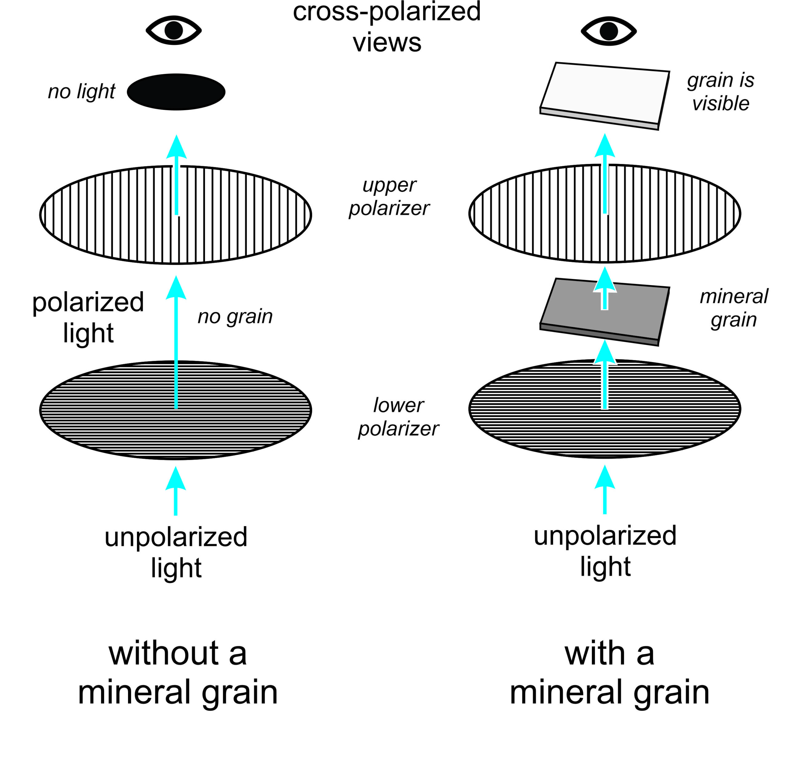
As pointed out previously, when viewing with the upper polarizer in place – under crossed polar (XP) light – we can differentiate isotropic and anisotropic crystals. If we are looking at an isotropic crystal using XP light, it will remain extinct (dark) through 360° of stage rotation. This is because the light emerging from the mineral retains the polarization it had on entering and will always be east-west polarized. It cannot pass through the upper polarizer, oriented at 90° to the lower polarizer. The effect is the same as if no mineral were on the stage.

But when we view an anisotropic crystal with XP light, light is split into two rays – a fast ray and a slow ray – unless we are looking down an optic axis (Figure 5.47). The two rays, after emerging from the crystal, travel on to the upper polarizer where they are resolved into one ray with north-south polarization. Because the vibration directions of the fast and slow rays are normally not perpendicular to the upper polarizer, only some components of both pass through the upper polarizer and combine to produce the light reaching our eye. As we rotate the microscope stage, however, the relative intensities of the two rays emerging from the crystal vary. Every 90°, the intensity of one is zero, and the other is vibrating perpendicular to the upper polarizer. Consequently, no light passes through the upper polarizer and the crystal appears extinct every 90°.

If we used a monochromatic light (one wavelength) source in our microscope and looked at an anisotropic crystal under XP light, it would go from light to complete darkness as we rotate the stage. Extinction would occur every 90°, and maximum brightness would be at 45° to the extinction positions. However, most polarizing microscopes use polychromatic light. Because of dispersion, double refraction is slightly different for different wavelengths. Minerals with high dispersion may never appear completely dark, but most come close.

▶️ Video 4: Explanation of double refraction with animation (2 minutes)

▶️ Video 5: What Happens at the Upper Polarizer? (3 minutes)

•Interference Colors

When white light passes through an anisotropic mineral, all wavelengths are split into two polarized rays vibrating perpendicularly. The slow ray lags behind the fast ray by a distance equivalent to the retardation. Different colors have different wavelengths, so when the rays leave the crystal, the fast and slow rays for any color may be in phase, completely out of phase or somewhere between depending on the retardation compared with wavelength (Figure 5.48). The waves will not initially interfere because they are vibrating in perpendicular directions and are not following the same paths. But when the north-south components of the two rays are combined at the upper polarizer (where the filter constrains them to vibrate north-south), constructive interference occurs for some colors, and destructive interference for others. Most wavelengths will not be completely in phase or out of phase, so some intermediate amount of interference will occur.

When we look at a mineral under XP light, we see one color. It is mostly a combination of those wavelengths that are in phase or partially in phase, and is missing wavelengths that are out of phase or mostly out of phase. Interference colors depend on the retardation of different wavelengths, which in turn depends on the orientation, birefringence, and thickness of a crystal. Interference colors change intensity and hue as we rotate the stage; they disappear every 90°, when the mineral goes extinct.

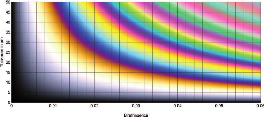
Retardation, and thus interference colors, vary with mineral birefringence and thickness. The Raith–Sørensen chart seen in Figure 5.49 shows the relationships. Retardation is proportional to birefringence and grain thickness, and it increases diagonally from zero in the bottom left corner to about 3,000 nm in the upper right corner.

Interference colors vary in hue and intensity with stage rotation, but this chart shows “maximum” interference colors that we may see halfway between extinctions. Grains that are very thin or that have very low birefringence display up to white interference colors. Those that are thicker and have greater birefringence display other colors. Overall, the colors become less pronounced as retardation increases.

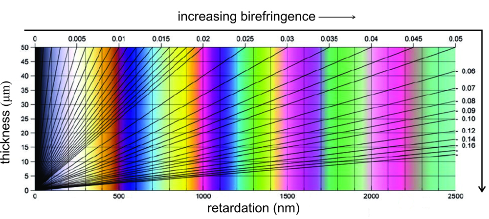
Figure 5.50 shows the same information as the previous figure but the axes have been changed. This kind of chart, called a Michel-Lévy Color Chart, is more commonly used by mineralogists than the Raith–Sørensen chart above. In a Michel-Lévy chart, the horizontal axis is retardation; it directly correlates with interference color (shown as vertical color swatches). The vertical axis is grain thickness. The diagonal lines and numbers on the top and right side of the chart show birefringence. (Birefringence was the horizontal axis in the Raith–Sørensen chart above in Figure 5.49.) Notice that the interference colors repeat hues, but become more washed-out (paler), as retardation increases.

Very low-order interference colors, corresponding to a retardation of less than 200 nm, are gray and white. If retardation is slightly greater, yellow, orange, or red interference colors will appear when we rotate the stage. These colors, corresponding to retardation of 200 nm to 550 nm, are called first-order colors. As retardation increases further, we see blue, and then colors repeat every 550 nm of retardation, the average wavelength of white light. This is because it does not matter if a wave is 1 wavelength, 2, or 3, behind another – it will still be in phase. And the same holds true for out-of-phase waves – it does not matter if they differ by 1.5, 2.5, etc., wavelengths, they are still out of phase.

So, colors go from gray to red (first order), from violet to red (second order) and then from violet to red again (third order), and continue to repeat. They become more pastel (washed out) in appearance as order increases. Fourth-order colors are often so weak that they appear “pearl” white (because they have a play of color like pearls) and may occasionally be confused with first-order white. So, when describing an interference color, stating both the color and the order is important. For mineral identification, the order is often more important than the color.

Birefringence can be a good tool for mineral identification. Standard thin sections are 30 μm (0.03 mm) thick but sometimes thin sections are poorly made, and often grains are thinner around their edges than in their centers. This chart reminds us that retardation, and thus interference colors, are a product of both thickness and birefringence. Additionally, birefringence depends on mineral orientation. If a mineral is oriented with an optic axis vertical, its birefringence will be zero. And if the optic axis is close to vertical, birefringence may be much less than the maximum it could be. Consequently, when estimating birefringence from interference colors seen in thin section, we must look at multiple grains of the same mineral to make sure we know what the maximum birefringence is.

Figure 5.51 shows PP and XP views of a thin section we saw earlier in this chapter. The rock contains mostly quartz, sillimanite and biotite. A few grains of opaque magnetite (black and unlabeled) are apparent in the PP view. Quartz has birefringence of about 0.01, biotite and sillimanite have greater birefringence. So the quartz shows only white and gray interference colors; the other minerals display bright blues, violets, yellows, and other hues.

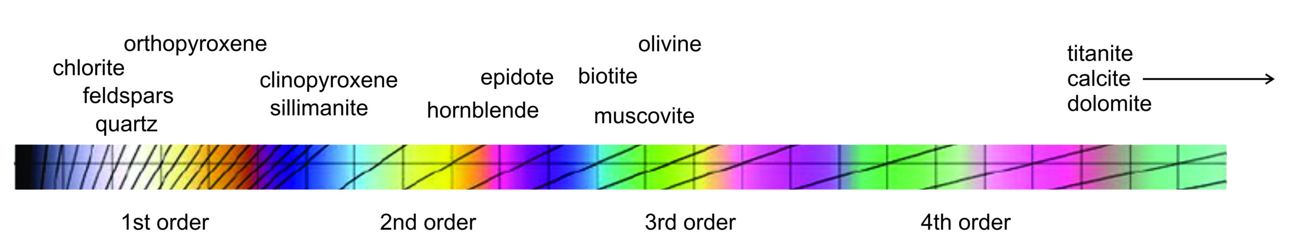
Figure 5.52, a slice through the Michel-Lévy chart in Figure 5.50, shows normal interference colors for some common minerals. If thin sections are of uniform thickness (30 μm) and minerals have normal compositions, these are the maximum interference colors that will be seen. Many complicating factors, including how well a thin section was made and the nature of the substage light source, can cause aberrations. Note that some relatively common minerals (titanite, calcite, and dolomite) plot way off-scale to the right on this diagram.

Minerals with very low birefringence that display first-order white, gray, or yellow interference colors include quartz, leucite, nepheline, apatite, beryl, and feldspar. Many other minerals have greater birefringence. For example, biotite and sillimanite, which have intermediate birefringence, display third-order colors. But, birefringence can be much greater.

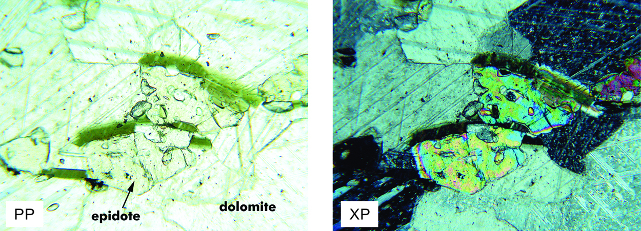
The epidote seen in Figure 5.53 (XP view) shows blotchy second- and third-order colors. Most of this specimen, however is dolomite. Dolomite has birefringence of about 0.2, which means its interference colors are off the chart – they are very high-order pearly pastels that appear almost white. Some minerals, including dolomite, titanite (sphene), and calcite have very high birefringence. So they commonly show such weak colors that it is impossible to estimate retardation and birefringence with any certainty.

Anisotropic minerals have different refractive indices that vary depending on the path light travels when passing through them. Their optical properties, including birefringence, and thus interference colors, depend on their orientation. For identification purposes, the maximum birefringence (δ), corresponding to the highest-order interference colors, is diagnostic. This may be hard to estimate in grain mounts because mineral thickness varies, making it difficult or impossible to estimate birefringence from interference colors. In thin sections, the task is easier because thickness is known (30 μm) so we can use the Michel-Lévy Chart to determine birefringence from interference color.

It is worth emphasizing that randomly oriented mineral grains may not show maximum interference colors. If minerals are oriented with an optic axis close to vertical, their birefringence may be much less than the maximum it could be. If the optic axis is vertical, the grain will appear extinct. Consequently, when estimating birefringence from interference colors seen in thin section, we must look at multiple grains of the same mineral to make sure we know what the maximum birefringence is. Because we cannot be exact, we normally use qualitative terms such as “low,” “moderate,” “high,” or “extreme” to describe retardation and birefringence.

•Anomalous Interference Colors

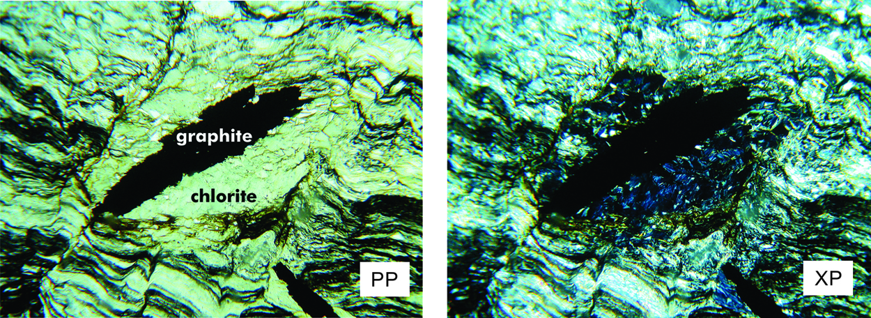
Some minerals display anomalous interference colors. These are colors not represented on the Michel-Lévy Color Chart. Anomalous interference colors may result if minerals have highly abnormal dispersion, if they are deeply colored, or for several other reasons. Minerals that commonly display anomalous inference colors include chlorite, epidote, zoisite, jadeite, tourmaline, and sodic amphiboles. Figure 5.54 shows a phyllite collected from near the Hudson River in Poughkeepsie, New York. In the PP view, chlorite appears drab and green, but in the XP view it displays inky blue interference color. Inky blue color, although not on the Michel-Lévy Chart, is often a key to identifying chlorite in thin section. Some chlorite, however, shows interference colors in other hues.

▶️ Video 6: Examples of low, medium, and high-order interference colors in thin section (3 minutes)

▶️ Video 7 summarizes fundamental information about interference colors (5 minutes)

•Twinning, Zoning, and Undulatory Extinction

Many minerals twin, and sometimes we can see the twins with a microscope. The dolomite in Figure 5.53, for example, shows stripes due to twinning in both the PP and the XP view. But normally we only see twinning when we cross the polars. Twins show in XP light because different twin domains have different crystallographic orientations. So the domains do not go extinct simultaneously when we rotate the microscope stage.

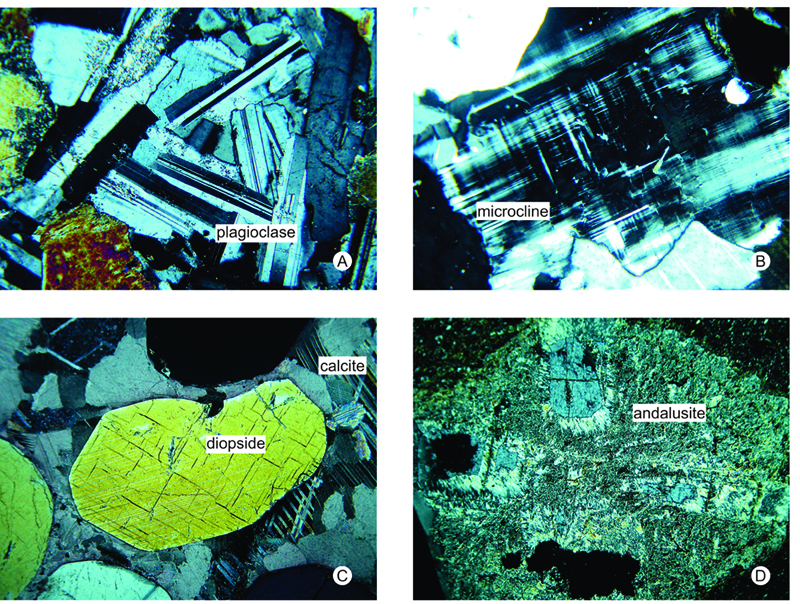
Figure 5.55 shows more examples of twinning. These are XP views of plagioclase, microcline, diopside, calcite, and andalusite. The plagioclase and diopside have lamellar twins (parallel with a long direction) and sharp twin boundaries (although the twins in the diopside are hard to see because they are so thin.) These are examples of contact twins. The calcite, microcline and andalusite grains contain penetration twins that cut across each other.

Twinning is often an excellent way to distinguish different minerals in thin section. Sometimes we describe plagioclase twinning (Figure 5.55a) as zebra stripes, for obvious reasons. The microcline (Figure 5.55b) shows two types of lamellar twins with different orientations. They combine to produce what we call microcline twinning or Scotch plaid twinning. Orthoclase (not shown) often contains simple contact twins. Calcite (Figure 5.55c) is characterized by polysynthetic twins parallel to the long diagonal of its rhombohedral shape. Other carbonates have no twins or have twins parallel to the short diagonal. The andalusite seen above (Figure 5.55d) contains a cross made by two twin domains – few minerals twin this way. Thus, for the feldspars, the carbonates, and for some other minerals, twinning can be a key to identification.

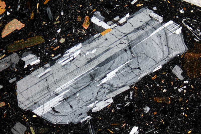
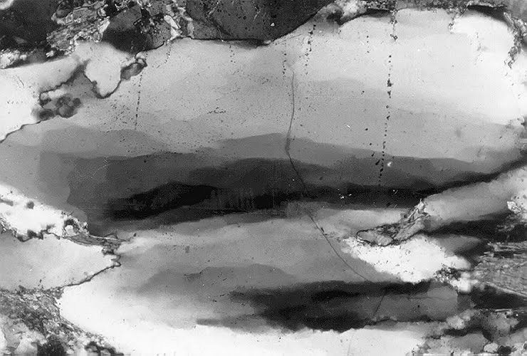
Some mineral grains, most notably those that crystallize from magma over a range of temperature, are heterogeneous. So different parts of grains have different optical properties, producing compositional zonation, commonly just called zoning. Feldspars and other minerals that commonly twin, often show zoning. Figure 5.56 is an example – a zoned plagioclase in rhyolite. The zoning appears as concentric rings that parallel the outside of the crystal, somewhat like tree rings. The rings developed as the grain crystalized from melt. Subsequently the mineral twinned, producing the long lathes parallel to the grain’s long dimensions. Many other minerals, besides plagioclase, can show zoning in thin section.

Quartz and some feldspars are known for displaying undulatory extinction when viewed under XP light. This kind of extinction is sometimes confused with compositional zonation. When a grain shows undulatory extinction, it means that different parts of a crystal go to extinction at different times with stage rotation. This gives an overall patchy or blotchy appearance. This property derives from strain imposed on a crystal after it formed. Undulatory extinction is so common in quartz that it is considered a diagnostic property. Figure 5.57 shows several large quartz grains. Portions of each are at extinction but most of the grains are not.

▶️ Video 8: twinning and zoning with some great photos (4 minutes)

5.5 More About Uniaxial and Biaxial Minerals

[In the discussion below, references are made to crystal systems and to crystallographic axes. But we do not talk about them in detail until later in this book. The interested reader will come back and read this section after having read Chapter 11.]

As described earlier in this chapter, if a crystal is oriented so that the optic axis is perpendicular to the microscope stage, light passing through the crystal travels parallel to the optic axis and behaves as if the crystal were isotropic. There is no double refraction and the polarization direction of the light is not changed by interaction with the crystal. If we view the crystal with the upper polarizer inserted (XP light) the grain will remain extinct even if we rotate the stage.

Most crystals in thin section, however, will not have optic axis vertical and we will see optical properties that relate to the crystal system of the mineral. For example, all minerals that have crystals belonging to the cubic crystal system are isotropic. They have the same light velocity and therefore the same refractive index (n) in all directions. The table below compares optical parameters and properties for isotropic, uniaxial, and biaxial minerals. Isotropic crystals have a single index of refraction (n) and their birefringence is zero.

Indices of Refraction and Birefringence in Isotropic and Anisotropic Crystals
	principle indices of refraction	index of refraction perpendicular to an optic axis	indices of refraction in a random direction	birefringence in a random direction	maximum possible birefringence
isotropic crystals uniaxial crystals biaxial crystals	n ω, ε α, β, γ	n ω β	n ω, εˈ αˈ, γˈ	0 δˈ = ∣ω – εˈ∣ δˈ = ∣γˈ – αˈ∣	0 δ = ∣ω – ε∣ δ = ∣γ – α∣

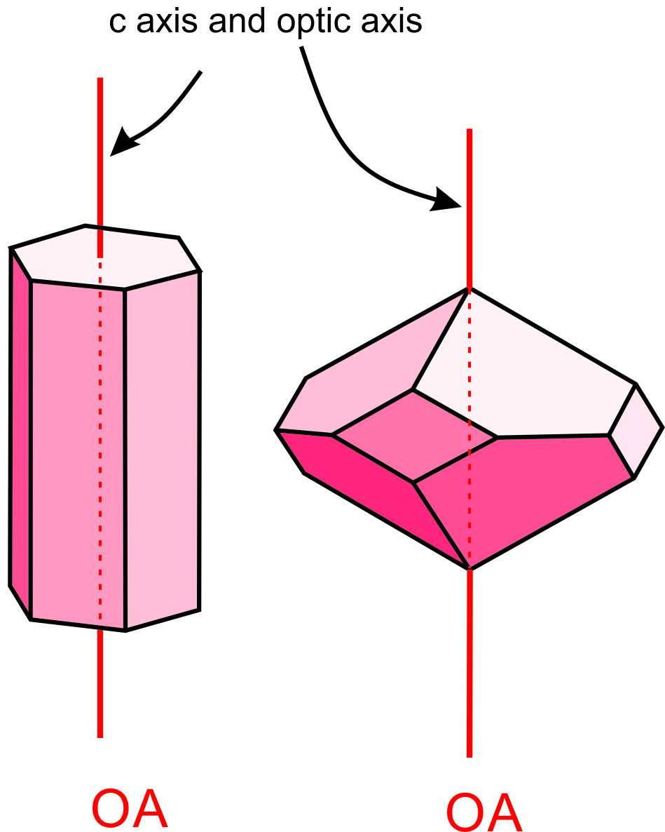
All minerals with crystals that belong to the tetragonal or hexagonal crystal systems are uniaxial, meaning that they have only one optic axis. In these crystals, the optic axis is coincident with the c crystallographic axis (Figure 5.58), and in many uniaxial minerals, the optic axis is parallel or perpendicular to crystal faces. In uniaxial crystals, refractive index varies between two limiting values, that we designate epsilon (ε) and omega (ω). The maximum value of birefringence in uniaxial crystals is the absolute value of the difference between ω and ε (see the table above): δ = |ω – ε|. We can only see maximum birefringence (which corresponds with maximum retardation) if the optic axis is parallel to the microscope stage.

Light traveling parallel to the single optic axis of a uniaxial mineral travels as an ordinary ray and has refractive index ω. Light traveling perpendicular to the optic axis has refracted index ε. Unless traveling parallel to the optic axis, light is doubly refracted, splitting into two rays with one having refractive index ω. The other ray has refractive index εʹ, which varies depending on the direction of travel. εʹ may have any value between ω and ε.

We divide uniaxial minerals into two classes: if ω < ε, the mineral is uniaxial positive ( + ). If ω > ε , the mineral is uniaxial negative (-). We can use the mnemonic POLE (positive = omega less than epsilon) and NOME (negative = omega more than epsilon) to remember these relationships. Positive minerals are often described as having a positive optic sign; negative minerals have a negative optic sign.

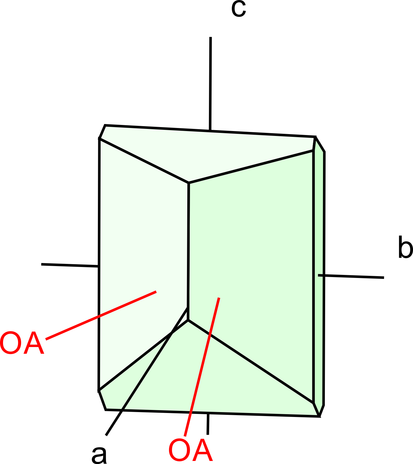
Biaxial minerals include all minerals that have crystals belonging to the orthorhombic, monoclinic, or triclinic systems. Biaxial crystals, such as the one shown in Figure 5.59, have two optic axes, and the axes are not coincident with crystallographic axes (a, b, or c). Like uniaxial crystals, biaxial crystals have refractive indices that vary between two limiting values. But, unlike uniaxial minerals, both limiting values change with changes in crystal orientation relative to the light source.

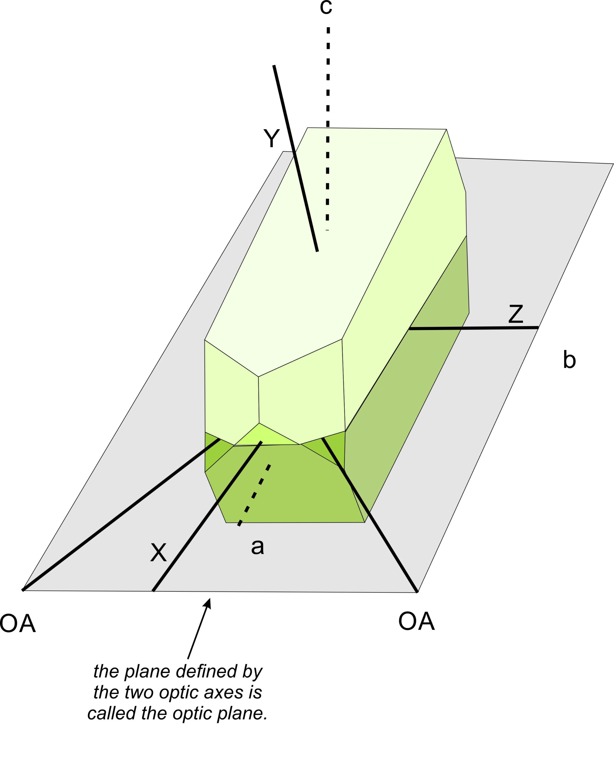
As with uniaxial crystals, light passing through a biaxial crystal experiences double refraction unless it travels parallel to an optic axis. We describe the optical properties of biaxial minerals in terms of three mutually perpendicular directions: X, Y, and Z (Figure 5.60).

The vibration direction of the fastest possible ray is designated X, and that of the slowest is designated Z. The indices of refraction for light vibrating parallel to X, Y, and Z are α, β, γ. α is therefore the lowest refractive index, and γ is the highest. β, having an intermediate value, is the refractive index of light vibrating perpendicular to an optic axis.

We divide biaxial minerals into two classes based on their refractive indices. In biaxial positive minerals, the intermediate refractive index β is closer in value to α than to γ. In biaxial negative minerals, it is closer in value to γ. Retardation and apparent birefringence vary with the direction light travels through a biaxial crystal, but the maximum value of birefringence (δ) in biaxial crystals is always γ – α. See the table above for descriptions of other parameters.

In orthorhombic crystals the optical directions X, Y, and Z correspond to crystal axes (a, b or c). But, it is not a one-to-one correspondence because the X direction can be either a, b, or c. The same holds for Y and Z. In monoclinic crystals either X, Y, or Z are the same as the b axis. For example, Figure 5.60 shows a monoclinic orthoclase crystal where z is equivalent to b. The other two optical directions do not correspond to crystal axes – but in many monoclinic crystals are close. In triclinic crystals there is no correspondence between optical axes and crystallographic axes.

Normally, light passing through a randomly oriented biaxial crystal is split into two rays, neither of which is constrained to vibrate parallel to X, Y, or Z, so their refractive indices will be some values between α and γ. However, if the light is traveling parallel to Y, the two rays have refractive indices equal to α and γ, vibrate parallel to X and Z, and the crystal will display maximum retardation. If the light travels parallel to an optic axis, no double refraction occurs, and it has a single refractive index, β. There is no birefringence or retardation and the mineral appears extinct.

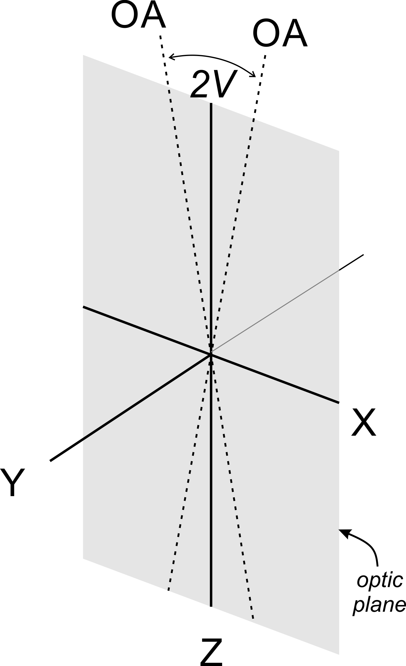
In biaxial minerals, we call the plane that contains X, Z, and the two optic axes the optic plane (Figures 5.60 and 5.61). The acute angle between the optic axes is 2V. A line bisecting the acute angle must parallel either Z (in biaxial positive crystals) or X (in biaxial negative crystals). We can measure 2V with a petrographic microscope and it can be an important diagnostic property. The feldspar in Figure 5.60 is biaxial negative but the drawing in Figure 5.61 is for a positive crystal.

5.5.1 Extinction Angles

Viewed with crossed polars, anisotropic grains go extinct every 90^o as we rotate the microscope stage. We can measure the extinction angle, the angle between a principal cleavage or direction of elongation (if the grain has a long dimension) and extinction by rotating the stage and using the angular scale around the stage perimeter.

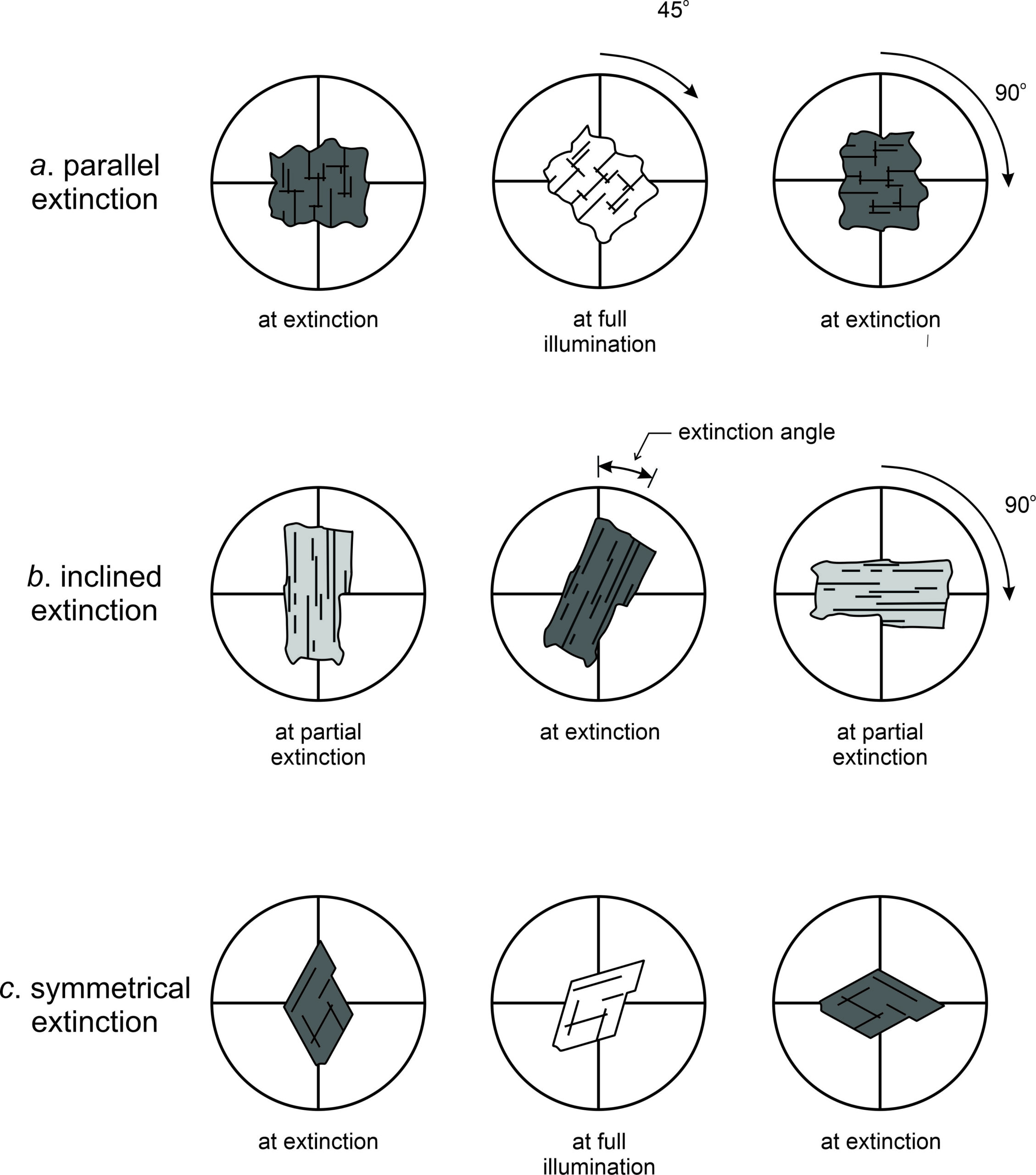
Some hexagonal, tetragonal, and orthorhombic minerals exhibit parallel extinction; they go extinct when their cleavages or directions of elongation are parallel to the upper or lower polarizer (Figure 5.62a). Many monoclinic and all triclinic crystals exhibit inclined extinction (Figure 5.62b) and go extinct when their cleavages or directions of elongation are at angles to the upper and lower polarizer. Some minerals exhibit symmetrical extinction; they go extinct at angles symmetrical with respect to cleavages or crystal faces (Figure 5.62c). These different kinds of extinction result from different kinds of atomic arrangements and so are diagnostic for mineral identification.

For any given mineral, the extinction angle seen in thin section depends on grain orientation. (This is because the apparent angle at which planes intersect depends on the direction of viewing.) But there is always some maximum value for any mineral. To determine this maximum value requires measurements on multiple grains, or on one grain in the correct orientation (determined by looking at interference figures, discussed later). If the grains are randomly oriented in a thin section and if the sample size is large enough, determining the maximum value is straightforward although, perhaps, a bit tedious.

5.5.2 Accessory Plates and the Sign of Elongation

We use accessory plates to make some measurements. When inserted, the slow and fast vibration directions of the plate are at 45° to the lower and upper polarizers. A double-headed arrow on accessory plates usually marks the slow direction. A standard full-wave plate has a retardation of 550 nm (equal to the average wavelength or visible light), equivalent to first-order red interference colors. A quartz wedge is sometimes a useful alternative to a full-wave plate. The wedge has a variable thickness, with retardation ranging from 0 nm to 3,500 nm. By inserting a plate or quartz wedge we add or subtract to the retardation of mineral grains.

Accessory plates make it possible to learn which vibration direction in a crystal permits polarized light to travel the fastest. If crystals have a long dimension, we can learn whether the mineral is length fast (also sometimes called negative elongation) or length slow (positive elongation). Determining the sign of elongation is often straightforward and can be helpful for identifying minerals.

Some anisotropic crystals have a prismatic or elongate habit, or a well-developed cleavage, that causes them to occur in elongated grains. Polarized light passing through a crystal with polarization parallel to the long dimension will not travel at the same velocity as light polarized in other directions. This distinction allows the minerals to be assigned a sign of elongation: length fast (faster light vibrates parallel to the long dimension) and length slow (slower light vibrates parallel to the long dimension). We cannot measure a sign of elongation for crystals that crystallize or cleave to produce equidimensional grains.

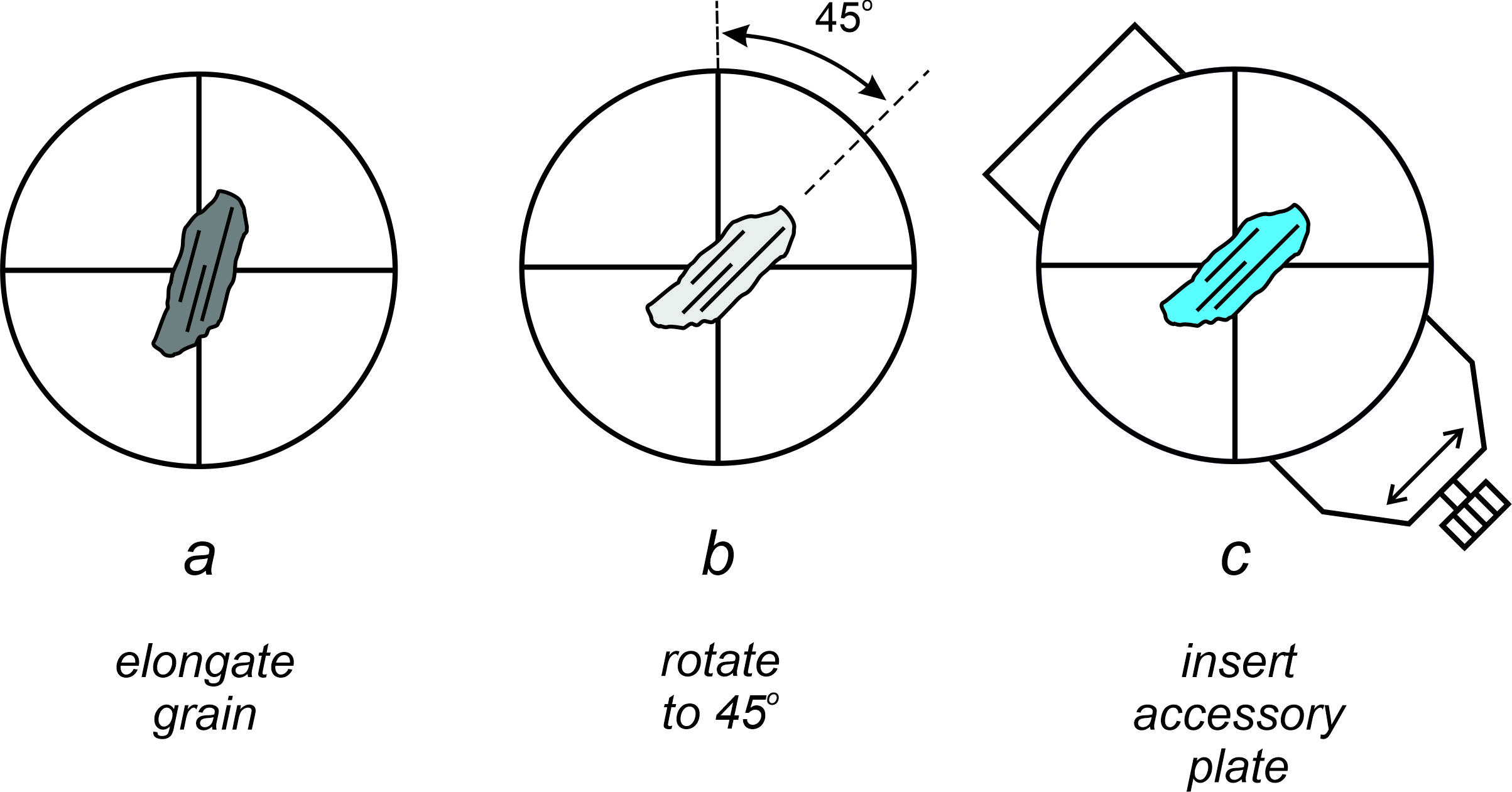
Determining the sign of elongation (length fast or length slow) is usually straightforward for tetragonal and hexagonal prismatic crystals (all of which are uniaxial) and some orthorhombic crystals. We orient the long dimension of a grain in a southwest-northeast direction (45^o to the polarizers) and note the interference colors (Figure 5.63). We then insert a full-wave accessory plate (having a retardation of 550 nm, equivalent to first-order red interference colors).

After insertion, the slow direction of most accessory plates will be oriented southwest-northeast. If the retardation of the accessory plates adds to the retardation of the grain, we get higher order interference colors, and the grain must be length slow. If retardation decreases, and we get lower-order colors, the grain must be length fast. Many minerals, especially if grains are small, exhibit low first-order interference colors (grays). If gray interference colors are added to first-order red, first-order blue results (Figure 5.63c). If gray interference colors are subtracted from first-order red, first-order yellow results. So, addition or subtraction is often just a matter of looking for blue or yellow. If we see blue or other higher-order interference colors when we insert the plate, the mineral is length slow (as in Figure 5.63c). If we see yellow or other lower-order colors, it is length fast.

If the interference colors for a mineral grain are not mostly gray, determining addition or subtraction may not be quite so simple. Sometimes we must rotate the stage to see the colors that appear when the mineral is oriented northwest-southeast. The effects in that orientation will be opposite to those seen when the mineral is oriented southwest-northeast. When oriented northwest-southeast, higher-order colors correspond to length fast, lower-order to length slow. A quartz wedge can be useful in determining the sign of elongation if a grain contains several color bands rather than just gray. If we insert the wedge in the accessory slot, the color bands on a southwest-northeast-oriented grain will move toward the thicker portions of the grain (usually the center of the grain) if the retardation is being subtracted (length fast). If the bands move away from the thicker portions of the grain, the retardation is being added (length slow).

Determining the sign of elongation for an orthorhombic, monoclinic, or triclinic mineral can be problematic or impossible. We can sometimes determine it for orthorhombic or monoclinic minerals with parallel extinctions, but it may vary with the orientation of the mineral. Mineral identification tables commonly list whether a given mineral is likely to provide a sign of elongation and whether the sign may vary with the mineral’s orientation. If the extinction angle of the monoclinic or triclinic grain is only a few degrees, we can often determine a sign of elongation. If they have inclined extinction, we often cannot make the determination because the sign may vary in a complicated way with the orientation of the grain, and because determining the orientation of the grain on the microscope stage is difficult.

5.6 Interference Figures

To determine whether an anisotropic mineral is uniaxial or biaxial, and whether it is optically positive or negative, requires obtaining an interference figure. Measuring 2V, for biaxial minerals, also requires an interference figure. We obtain these figures using a conoscopic lens below the microscope stage, and a Bertrand lens above the upper polarizer, when looking at a grain with XP light. Figure 5.23 shows this arrangement.

Any uniaxial or biaxial mineral (whether in a grain mount or a thin section) will, in principle, produce a visible interference figure; isotropic minerals will not. We must take care to choose grains without cracks or other flaws so light can pass through without disruption. In addition, for some purposes, we need grains with a specific orientation.

Having chosen an appropriate grain, obtaining an interference figure is relatively straightforward. We focus the microscope using PP light and high magnification. (If perfect focus is ambiguous, it often helps to focus first at low magnification.) Then we insert the upper polarizer to get XP light. If the microscope is properly aligned, the grain will still be in focus. Next, we fully open the substage diaphragm, insert the substage conoscopic lens (if it is not already in place), and then insert the Bertrand lens above the upper polarizer.

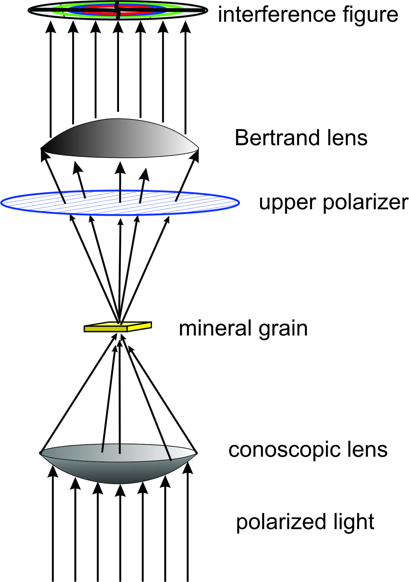
As seen in Figure 5.64, the conoscopic lens focuses polarized light so it enters a mineral grain from many different angles simultaneously and focuses on a small area. Double refraction occurs for all rays and different wavelengths have different retardations. At the upper polarizer, slow rays and fast rays combine to produce interference colors. And above that polarizer, the Bertrand lens focuses the light so it is parallel again. The Bertrand lens also magnifies the image.

So, the two special lenses together permit us to see an interference figure and examine light traveling through a crystal by many paths in a single view. Without the lenses, we would have to look at many different crystals to obtain the same information. (Some older microscopes do not have Bertrand lenses, but we can still see an interference figure by removing an ocular and inserting a peep sight, or by just peering down the tube. The figures, however, will be quite small.)

5.6.1 Uniaxial Interference Figures

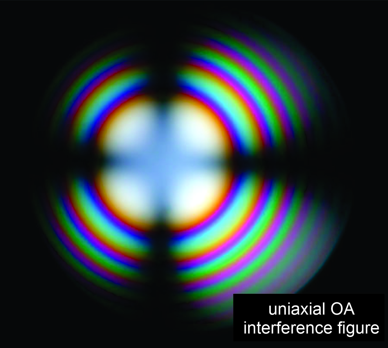
The best way to learn the optic sign of a uniaxial mineral, is to obtain an interference figure looking down, or nearly down, a crystal’s optic axis. The figure obtained is an optic axis (OA) figure; Figure 5.65 shows an example. Finding a grain that gives an OA figure is normally not difficult. Grains oriented with the optic axis vertical appear isotropic (when viewed under normal XP light) because they produce no double refraction. Grains oriented with the optic axis close to vertical have low retardation and, therefore, low-order interference colors.

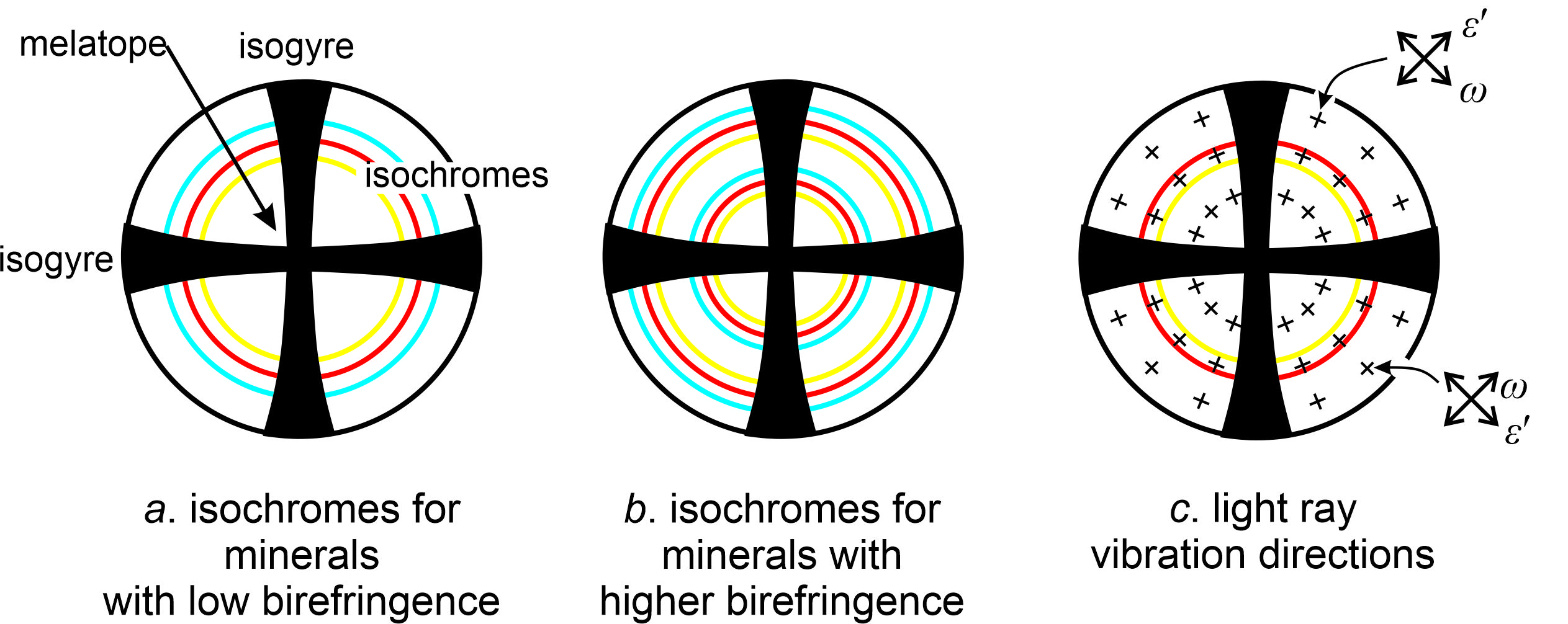
A centered uniaxial OA figure contains a black cross, like the one seen in the photo above (Figure 5.65), and depicted in Figure 5.66a, b and c. The cross will not move much if we rotate the stage. The center of the cross, called the melatope, corresponds to the direction of emergence of the optic axis. We call the dark bands forming the cross isogyres. The surrounding colored rings, if present, are isochromes. They are bands of equal retardation caused by the light entering the crystal at different angles (because of the conoscopic lens). Interference figures for minerals with very low birefringence, like quartz and feldspars, may not show any colored isochromes but most minerals do. Minerals with low to moderate birefringence typically show a few isochromes (Figure 5.66a), and interference figures for minerals with high birefringence commonly show many (Figure 5.65 and Figure 5.66b).

As shown in Figure 5.66c, in all parts of a uniaxial optic axis interference figure εʹ vibrates radially (along the radius of the interference figure) and ω vibrates tangent to isochromes. One way to remember these relationships is with the acronym WITTI for the mnemonic “ω is tangent to isochrome.”

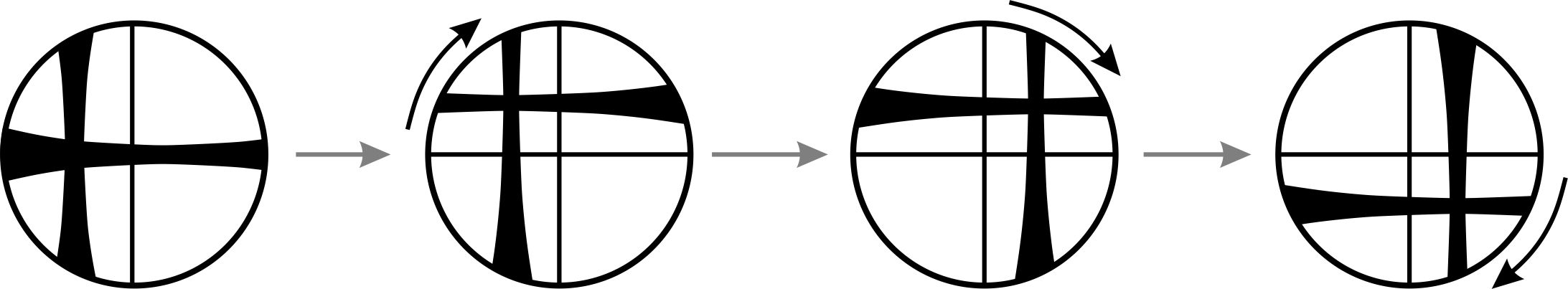
Sometimes, we obtain an optic axis figure but the optic axis is not perfectly vertical. If so, the black cross will be off center. As we rotate the stage the cross will precess as the melatope follows a circular path (Figure 5.67). The two links below will take you to short videos showing uniaxial interference figures precessing during stage rotation. But, even if the interference figure is somewhat off center, we can use it to learn the optic sign. And once we have an OA figure, perfectly centered or not, we use an accessory plate to learn whether a mineral is positive or negative. We describe this procedure below.

▶️ Video 9: Short video showing an optic axis figure for calcite changing during stage rotation (15 seconds)

▶️ Video 10: Short video showing and optic axis figure for benitoite changing during stage rotation (30 seconds)

Caveat: Most randomly oriented uniaxial mineral grains do not exhibit a centered OA figure. The optic axis is only one direction in the crystal and grains are unlikely to have their optic axis vertical. If the optic axis of a grain lies parallel to the stage of the microscope, we get an optic normal figure, also called a flash figure. The flash figure appears as a vague cross or blob that nearly fills the field of view when the grain is at extinction (when the optic axis is perpendicular to a polarizer). Upon stage rotation, it splits into two curved isogyres flashing in and out of the field of view with a few degrees of stage rotation. Biaxial flash figures have the same general appearance.

5.6.1.1 Determining the Optic Sign of a Uniaxial Mineral

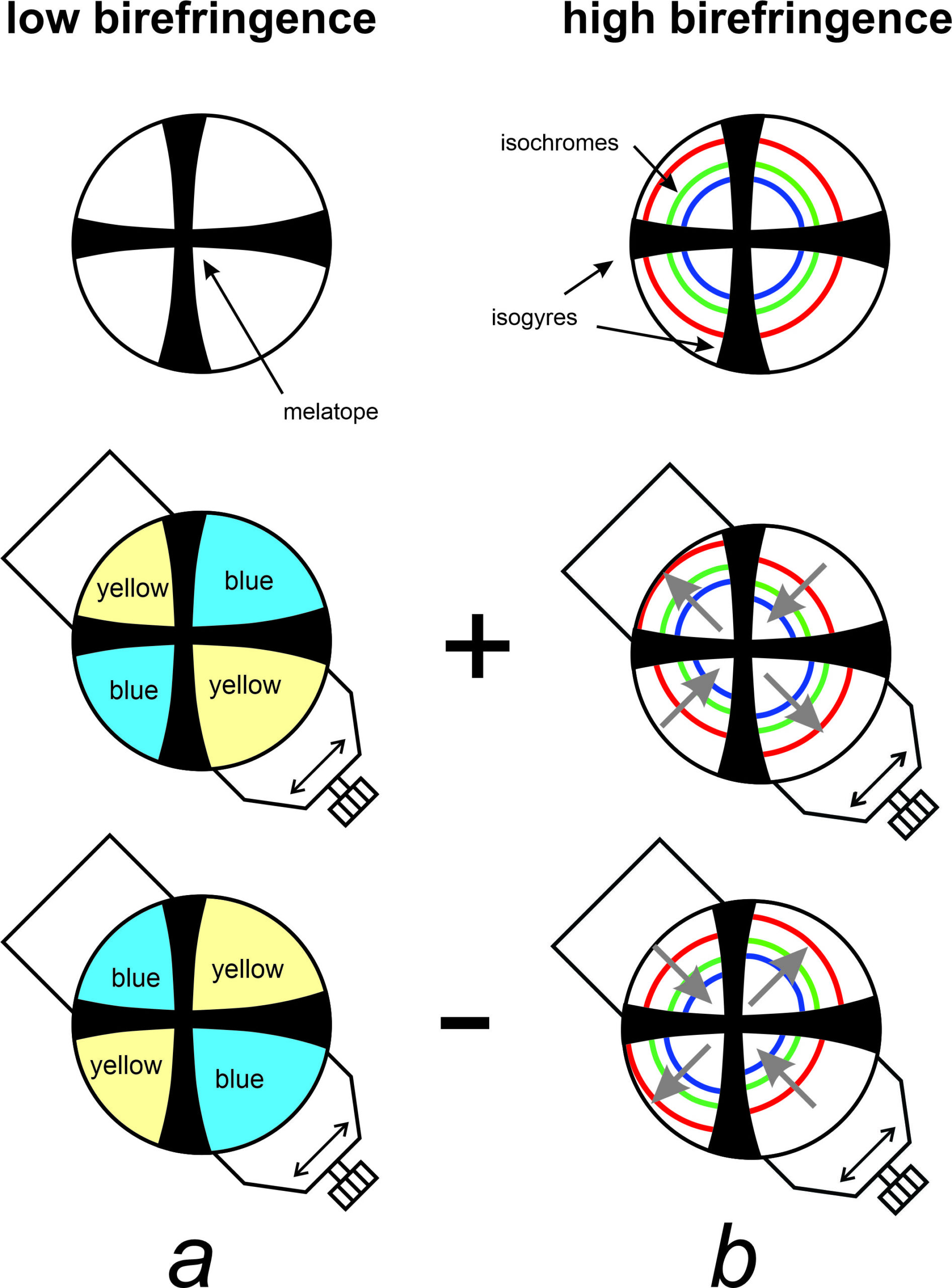
To know the optic sign of a uniaxial mineral, we must determine whether ω > ε or ε > ω. We make this determination by examining an optic axis figure and using an accessory plate with known orientation of the fast and slow rays. Standard accessory plates have their slow direction oriented southwest-northeast at 45° to both polarizers. We insert the plate, and we observe interference color changes or isochrome (color ring) movements in the southwest and northeast quadrants of the interference figure (Figure 5.68).

If the slow direction of the accessory plate corresponds to the slow direction of the mineral, retardation will add and we will see higher order interference colors. If they do not correspond, retardation will, in part, cancel and we will see lower order colors. In a uniaxial optic axis figure, εʹ vibrates radially. So, if interference colors in the southwest and northeast quadrants shift to higher orders when we insert the plate (or wedge), addition of retardation has occurred. So, εʹ is the slow ray and the crystal is uniaxial positive. Subtraction (lower-order interference colors) in the southwest and northeast quadrants indicates that εʹ is the fast ray, and the crystal is optically negative. Because εʹ vibrates parallel to the prism axis (c-axis) in prismatic uniaxial minerals, the optic sign is the same as the sign of elongation.

Although we could use a quartz wedge, we normally use a full-wave accessory plate when the optic axis figure shows low-order interference colors. In positive crystals, addition produces light blue in the southwest and northeast quadrants of the interference figure (Figure 5.68a), while subtraction produces light yellow in the northwest and southeast quadrants. In negative crystals, the effect is the opposite. If several different color rings (isochromes) are visible, the blue and yellow colors will only appear on the innermost rings near the melatope (the center of the black cross).

We can sometimes use a full-wave plate, but normally use a quartz wedge, to learn an optic sign for minerals that exhibit high-order interference colors. The retardation of the quartz will add to the retardation of the unknown mineral in two quadrants as we insert the wedge. It will also subtract from the retardation in the other two. The result will be color rings (isochromes) moving inward in quadrants where addition occurs, and outward in quadrants where subtraction occurs (Figure 5.68b). For positive minerals, this means that colors move inward in the southwest and northeast quadrants and outward in the northwest and southeast quadrants. For negative minerals, the motion is opposite.

5.6.2 Biaxial Interference Figures

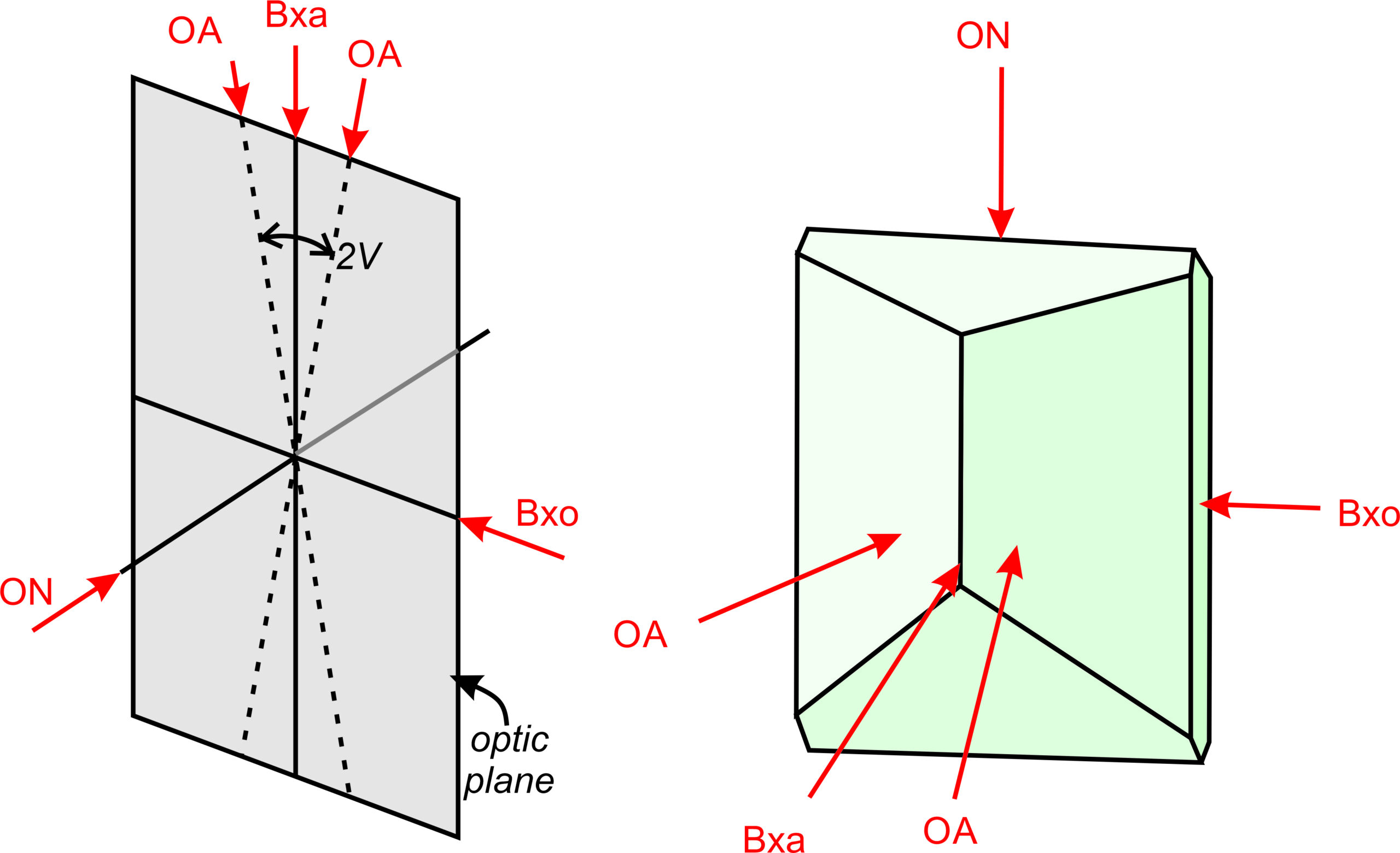
We obtain biaxial interference figures in the same way as uniaxial interference figures. However, complications arise with biaxial minerals because it is more difficult to find and identify grains oriented in a useful way. We can get interference figures from all grains, but interpreting them can be difficult or impossible.

With care, however, we can identify three different kinds of useful figures: optic axis figures (OA), acute bisectrix figures (Bxa), and optic normal figures (ON). Each corresponds to a different light path through the crystal, relative to the orientation of the optic axes. A fourth type of figure – a Bxo figure (Bxo) – is generally of limited use but we discuss it briefly in the interests of thoroughness.

Figure 5.69 shows the orientations of the different views for a typical biaxial mineral. The optic plane is vertical in the drawing on the left, but is horizontal in the drawing on the right. You can compare these drawings with ones seen earlier in which the crystallographic (a, b, c) and optical axes (X, Y, and Z) were labeled (Figures 5.60 and 5.61).

▶️ Video 11: Biaxial interference figures with good photos (5 minutes)

5.6.2.1 Optic Axis Figure

We obtain an OA figure by looking down an optic axis (Figure 5.69). We can find grains oriented to give an OA figure because they have zero or extremely low retardation. Under normal XP light, they remain dark even when we rotate the microscope stage. An interference figure will show only one isogyre unless 2V is quite small (less than 30°).

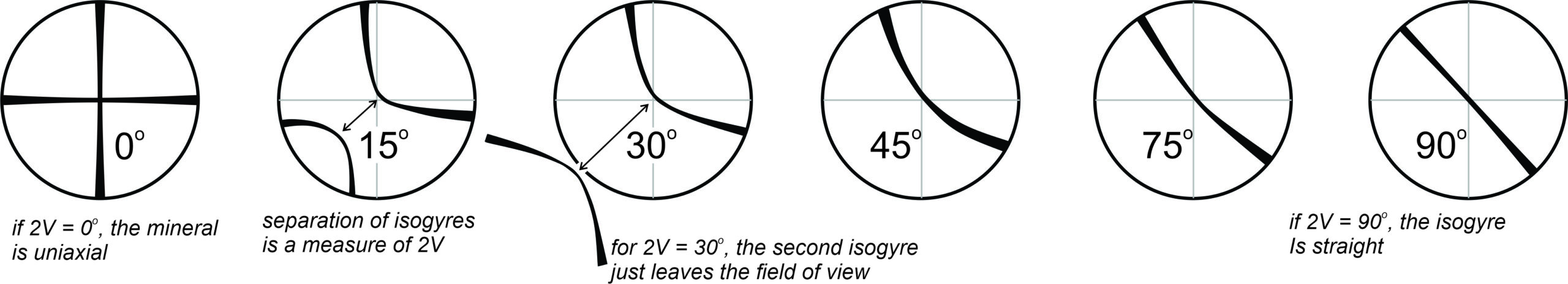
Figure 5.70 show depictions of isogyres for different values of 2V. (In these drawings, the isogyres are narrow with sharp boundaries but in thin section they are commonly quite diffuse.) No matter the 2V value, if the figure is perfectly centered, the isogyres will remain centered with stage rotation. If 2V = 0^o it means we are looking at a uniaxial mineral and we see a black cross. If 2V is very low (< 30̊^o) We will see two isogyres, shown in the 15^o drawing above. The two isogyres will come together and separate with stage rotation. If 2V > 30^o the second isogyre no longer enters the field of view. As 2V approaches 90^o, the single isogyre becomes straighter, and at 90^o the isogyre is completely straight. So, the curvature allows us to estimate 2V.

For any value of 2V, stage rotation causes isogyre rotation. For some purposes, discussed later, we may wish to know which side of the isogyre is concave and which is convex; this can be difficult to discern if 2V is very large because the isogyre will be nearly straight. In part also, the difficulty arises because a straight biaxial isogyre (unlike a uniaxial isogyre) does not have to be parallel or perpendicular to the microscope crosshairs.

▶️ Video 12: Link to an optic axis figure for betrandite (biaxial) (30 seconds)

5.6.2.2 Bxa and Bxo Figures

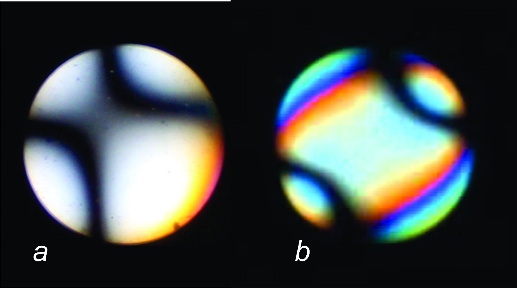
We obtain Bxa figures, such as those in Figure 5.71 by looking down the acute bisectrix, the line bisecting the acute angle between the two optic axes (Figure 5.69). We obtain a Bxo figure by looking down the obtuse bisectrix, the line bisecting the obtuse angle between the two optic axes (Figure 5.69). In biaxial positive crystals, Bxa corresponds to a view along Z; in biaxial negative crystals, it corresponds to a view along X. The opposite is true for Bxo figures. Generally, however, we do not seek a Bxo figure because it is of less use than a Bxa. So the discussion below focuses mostly on Bxas.

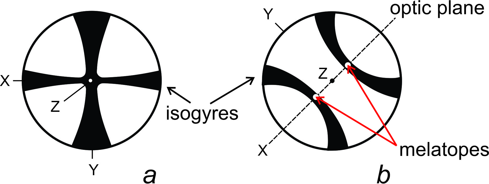
When we observe an acute bisectrix figure (Bxa) for a grain in an extinction orientation (which occurs when Y is perpendicular to a polarizer), it appears as a black cross, similar in some respects to a uniaxial interference figure (Figure 5.72a). When we rotate the stage, the cross splits into two isogyres that move apart and may leave the field of view (Figure 5.72b). After a rotation of 45°, the isogyres are at maximum separation; they come back together to reform the cross every 90°.

The points on the isogyres closest to the center of a Bxa (or a Bxo), the melatopes, are points corresponding to the orientations of the optic axes (Figure 5.72b). (Figure 5.72b is for a biaxial positive crystal; X and Z will switch places for a biaxial negative crystal.) If the retardation of the crystal is large enough, isochromes circle the melatopes. Some colorful isochromes are apparent in Figure 5.71b, above. Isochrome interference colors increase in order moving away from the melatopes because retardation is greater as the angle to the optic axes increases.

In Figure 5.71a, the isogyres are just beginning to separate; in Figure 5.71b they are at maximum separation. The maximum amount of isogyre separation depends on 2V; the greater the separation, the larger the 2V. If 2V is less than about 60°, the isogyres of a well-centered figure stay in the field of view as we rotate the stage. If 2V is greater than 60°, the isogyres completely leave the field of view

Finding a grain that yields a Bxa is easiest for minerals with a small 2V. We begin by searching for a grain that has minimal retardation. Such a grain will be oriented with an optical axis near vertical. Then we obtain an interference figure. We rotate the stage, and note how the isogyres behave. After checking several grains, we will find a Bxa. For minerals with low-to-moderate 2V, both isogyres will stay in the field of view, but the interference figure may not be perfectly centered. If an isogyre leaves the field of view, we check other grains until we are sure we are looking at a nearly centered Bxa. Getting a perfectly centered Bxo or Bxa figure can be, however, difficult and, sometimes for off-centered figures, we may only see one isogyre clearly.

For minerals with high 2V, the search for a Bxa sometimes becomes frustrating. Distinguishing a Bxa from a Bxo may be difficult or impossible. If we mistake one for the other, we may get some properties, 2V for example, wrong if we make measurements. But, the isogyres in a Bxo figure always leave the field of view because, by definition, an obtuse angle separates the optic axes in the Bxo direction. Thus, if the isogyres remain in view, the figure is a Bxa figure. For standard lenses, if the isogyres leave the field of view, the figure may be a Bxo or a Bxa for a mineral with high 2V (greater than about 60°). Expert optical mineralogists can tell a Bxa from a Bxo figure by the speed with which the isogyre leaves the field of view on stage rotation. For the rest of us, it is probably best to search for another grain with a better orientation.

▶️ Video 13: Link to off-center Bxa figure for titanite (30 seconds)

▶️ Video 14: Link to Bxa video for phlogopite (30 seconds)

5.6.2.3 Optic Normal Figure (ON)

We get an optic normal (ON) figure by looking down Y, normal to the plane of the two optic axes (see Figures 5.60 and 5.61). Grains that yield an optic normal figure are those that have maximum retardation, which means maximum interference colors. The interference figure resembles a poorly resolved Bxa, but the isogyres leave the field of view with only a slight rotation of the stage. Biaxial optic normal figures appear similar to uniaxial flash figures.

5.6.2.4 Determining Optic Sign and 2V of a Biaxial Mineral

Determining optic sign from a Bxa figure is equivalent to asking whether the Bxa view is parallel to the fast direction (biaxial negative crystals) or to the slow direction (biaxial positive crystals). We can often make the determination in much the same manner as for a uniaxial optic axis figure. However, for figures where the isogyres leave the field of view, this is not the recommended method because we can easily confuse Bxa and Bxo figures when 2V is greater than 70° or 80°. An alternative way to learn optic sign and 2V is to find a grain that yields a centered optic axis figure. Finding such grains is often not difficult because they show very low-order interference colors, or may appear isotropic under crossed polars. Below, we discuss both methods.

5.6.2.5 Determining Sign and 2V from a Bxa Figure

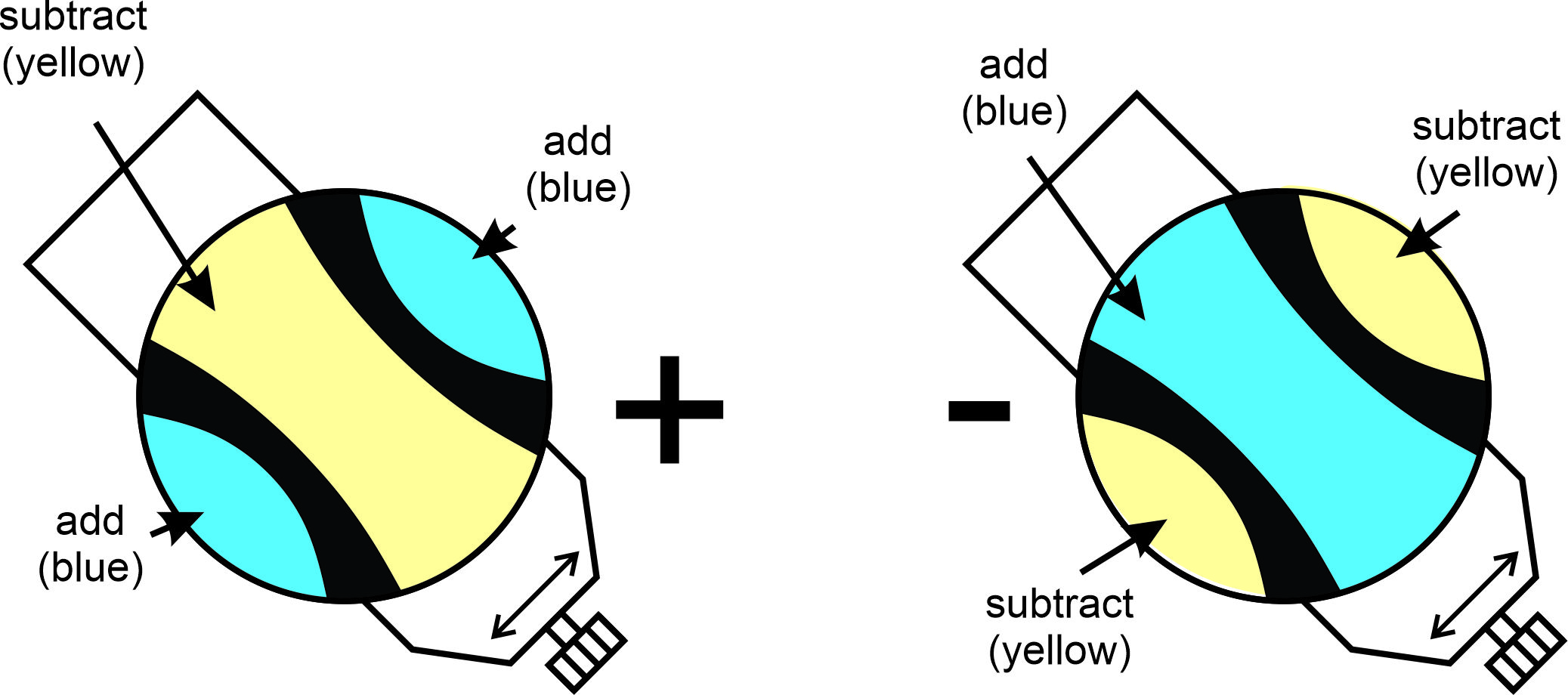
To measure optic sign and 2V using a Bxa figure, we rotate the stage so the isogyres are in the southwest and northeast quadrants (Figure 5.73). The Y direction in the crystal is now oriented northwest-southeast. The points corresponding to the optic axes (the melatopes) are the points on the isogyres closest to each other, and either X or Z is vertical depending on optic sign.

To determine optic sign, we must know which direction (X or Z) is vertical, corresponding to Bxa. If the slow direction (Z) corresponds to Bxa, the crystal is positive. If the fast direction (X) is Bxa, the crystal is negative. To make the determination, we insert the full-wave accessory plate (with slow-oriented direction southwest-northeast) and note any changes in interference colors on the concave sides of the isogyres. If the interference colors add on the concave sides of the isogyres (and subtract on the convex sides), the mineral is positive (Figure 5.73).

In positive minerals with low to moderate retardation, the colors in the center of the figure will be yellow (subtraction), and those on the concave side of the isogyres will be blue (addition). In a negative mineral, the color changes will be the opposite. For minerals with high retardation, it may be difficult to decide whether a full-wave accessory plate adds or subtracts retardation because isochromes of many repeating colors circle the melatopes. A quartz wedge simplifies determination. As we insert the wedge, color rings move toward the melatopes if there is addition of retardation, or the rings move away from the melatopes if there is subtraction. If the interference colors move toward the optic axes from the concave side of the isogyres, and away on the convex side, the mineral is positive. We see the opposite effect for a negative mineral.

We can estimate 2V from a well-centered Bxa figure by noting the maximum of separation of the isogyres during stage rotation. For standard lenses, if the isogyres just leave the field of view when they are at maximum separation, 2V is 60° to 65°. If the isogyres barely separate, 2V is less than about 10°.

5.6.2.6 Determining Sign and 2V from an Optic Axis Figure

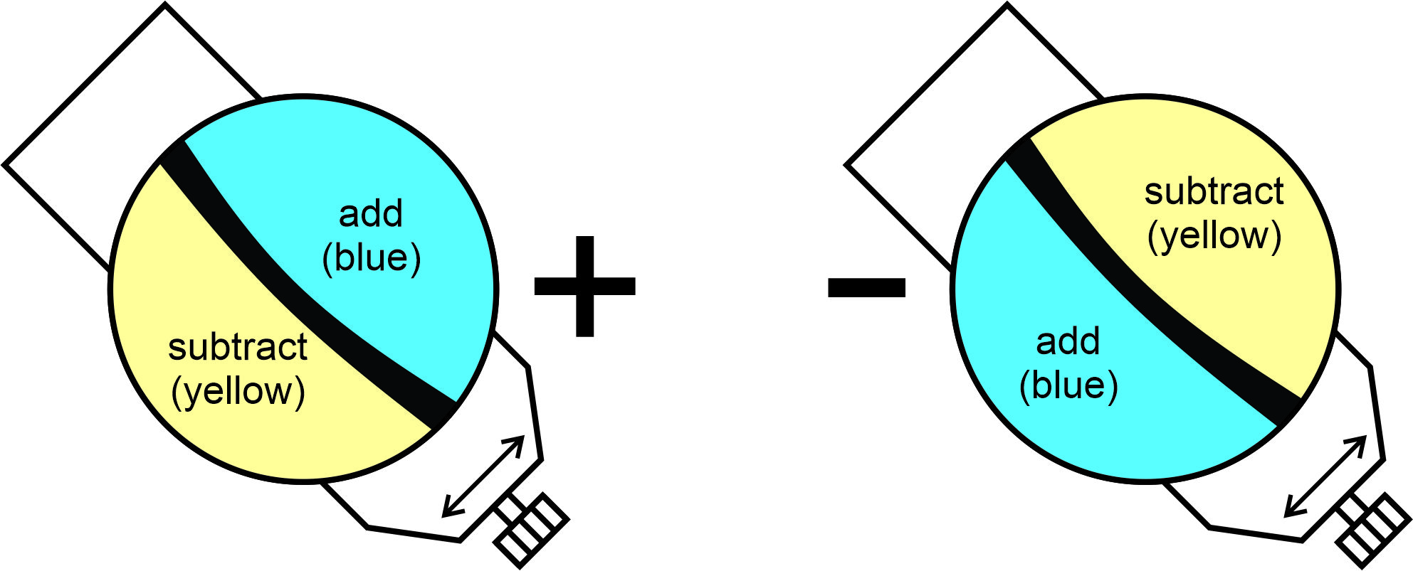
Determining the optic sign from an optic axis figure can often be simpler than looking for a Bxa. To find an OA figure, we look for a grain displaying zero or very low retardation. Once we have an interference figure, we rotate the stage and we should see one centered or nearly centered isogyre (Figures 5.70). (If, instead, we see two isogyres that stay in the field of view when we rotate the stage, we are looking at a Bxa for a mineral with low 2V.) We rotate the stage so the isogyre (or the most nearly centered if there are two isogyres) is concave to the northeast (Figure 5.74). Note that isogyres rotate in the opposite sense from the stage.

We then insert the full-wave accessory plate. If the retardation increases on the concave side of the isogyre (and decreases on the convex side), the mineral is positive (Figures 5.74). In minerals with low to moderate retardation, we need only to look for yellow and blue. Blue indicates an increase and yellow a decrease in retardation. The increase or decrease of retardation will be opposite if the mineral is negative.

We estimate 2V by noting the curvature of the isogyre. If 2V is less than 10° to 15°, the isogyre will seem to make a 90° bend. If 2V is 90°, it will be straight. For other values, it will have curvature between 90° and 0° (Figure 5.70).

5.7 Identifying Minerals and Mineral Properties in Thin Section

Learning to identify minerals in thin section takes practice. But, if we have a hand specimen or know what kind of rock we are looking at, the most likely possibilities are limited – and identification is simplified. And some common minerals have key properties that make identification straightforward. So, just like identifying hand specimens based on physical properties, it is not always necessary to check or measure every optical property to figure out what a mineral is. To see photos of the most common minerals in thin section with a discussion of key properties that aid identification, go to our website Optical Mineralogy. For many more, and higher quality photographs of minerals in thin section, go to Frank Mazdab’s rockPTX.com website, or to Alessandro Da Mommio’s website at www.alexstrekeisen.it/english/.

With the above said, a standard approach works well. This approach involves looking at multiple grains of each mineral and changing back and forth between plane polarized (PP) and crossed polarized (XP) light. Sometimes we need an interference figure. But for routine mineral identification, obtaining an interference figure is often unnecessary and identification can be quite rapid. The flow chart in Box 5-4 below summarizes the key steps and questions to ask as you go along. If you do all that is described and you still cannot identify a mineral, you have been very unlucky.

● Box 5-4  Identifying Minerals and Measuring Mineral Properties with a Polarizing Microscope 1. Look at the whole thin section (and at a hand specimen if available): • What kind of rock is it? • How many different major minerals does it contain? • What are the associated minerals? 2. Examine several grains of the same mineral under PP light: • Is the mineral opaque or nonopaque? • What color is the mineral? Rotate the stage. • Is it pleochroic? • What is the color variation? • What is the crystal shape and habit? • What cleavage does it display, if any? • What is its apparent relief? 3. Now cross the polars to examine several grains of the same mineral under XP light: • Rotate the stage. Is the mineral isotropic or anisotropic? 4. If anisotropic: • Rotate the stage. What is the range of interference colors? • Estimate the maximum birefringence by looking at grains with the highest order of interference colors. • For minerals with a long dimension of principal cleavage: What is the maximum extinction angle? • Is the mineral length fast or length slow ? • Is the mineral twinned? If so, what kinds of twins? 5. If necessary, obtain an interference figure. You may have to try several different grains to get one that is useful: • Is the mineral uniaxial or biaxial? • What is its optic sign? 6. If biaxial: • Estimate 2V.

 

 

●Figure Credits Uncredited graphics/photos came from the authors and other primary contributors to this book. 5.2 Microscope lenses and a thin section, “Introduction to Petrology” by Johnson, E.A., Liu, J. C., and Peale, M., https://viva.pressbooks.pub/petrology 5.3 Fractured grains of garnet, lobotka.net 5.5 Ore from Butte, Montana, Eastman (2017) 5.8 Wavelengths and colors of visible light, caltechletter.org 5.10 Light refraction, ucar.edu 5.13 Light dispersion, Cepheiden, Wikimedia Commons 5.14 Diamond dispersion, thoughtco.com 5.18 Looking at fish, shadesdaddy.com 5.25 Angular scale on a microscope, Johnson et al. (ibid) 5.26 Microscope turret, Johnson et al. (ibid) 5.27 Microscope eyepieces, Johnson et al. (ibid) 5.28 Quartz wedge and accessory plates, Johnson et al. (ibid) 5.35 Garnet and halite, lobotka.net. 5.36 Grains in refraction oil, sun.ac.za 5.39 Becke lines, gemsandmineralacademy.files.wordpress 5.45 Iceland spar (geologypics.com) 5.49 Raith–Sørensen chart, Sorensen (2013) 5.50 Michel-Lévy chart, Sorensen (2013) 5.56 Plagioclase in rhyolite, alexstrekeisen.it 5.57 Quartz in thin section, pinterest.com 5.65 Uniaxial optic axis figure, jm-derochette.be Video 2: Becke lines, Brent Owens Video 7: Interference colors, Johnson et al. (ibid) Video 8: Twinning and zoning, unknown origin Video 9: Calcite interference figure, AmiGEO Video 10: Benitoite interference figure, Frank Mazdab Video 11: Biaxial interference figures, Johnson et al. (ibid) Video 12: Optic axis figure – bertrandite, Frank Mazdab Video 13: Bxa figure – titanite, Frank Mazdab Video 14: Bxa figure – phlogopite, Frank Mazdab