11 – Crystallography
KEY CONCEPTS
- All crystals are made of basic building blocks called unit cells.
- Unit cells may have any of 7 fundamental shapes.
- Unit cells fit together in one of 14 ways to make crystals.
- We make inferences about unit cell shape and lattice type based on crystal habit and symmetry.
- The symmetry of an atomic structure depends on unit cell shape, the lattice, and the locations of atoms in the unit cell.
- There are 230 possible atomic-structure symmetries that can only be distinguished using X-ray techniques.
- Crystals contain one or several different kinds of crystal faces.
- We differentiate crystal faces based on their orientations with respect to a coordinate system based on unit cell edges.
11.1 Observations in the Seventeenth through Nineteenth Centuries
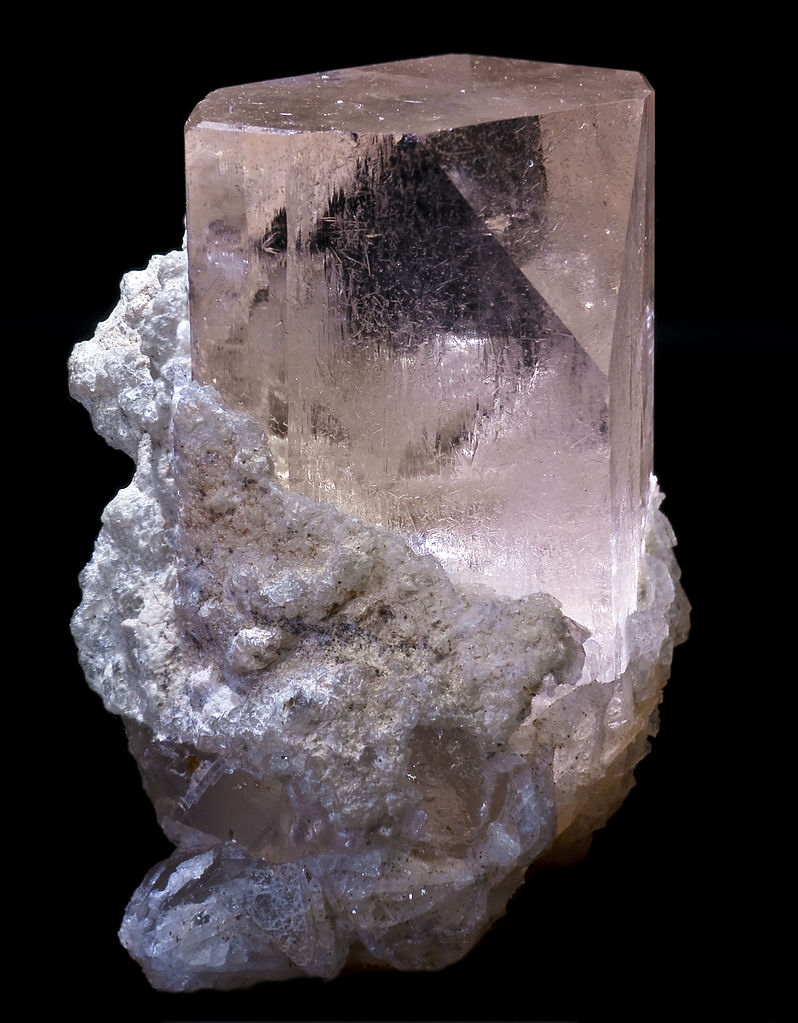
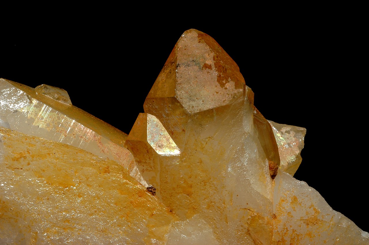
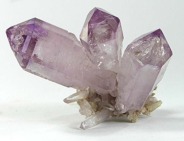
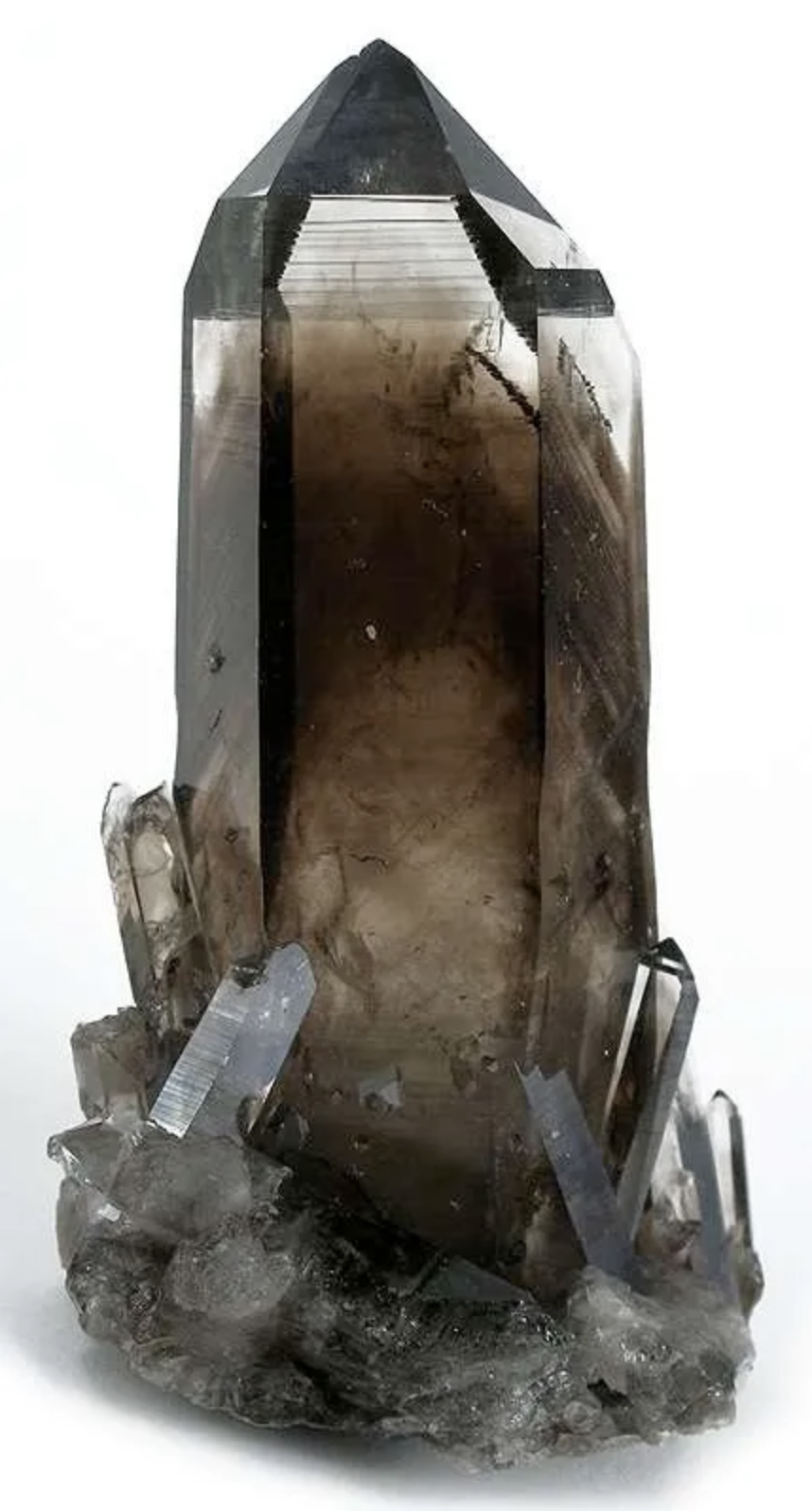
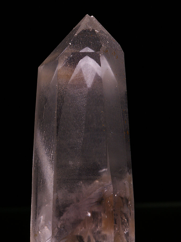
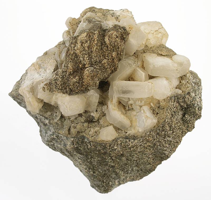
In 1669 Nicolaus Steno studied many quartz crystals and found angles between adjacent prism faces, termed interfacial angles, to be 120o no matter how the crystals had formed. For example, Figures 11.2 to 11.5 show four varieties of quartz with nearly identical crystal shapes and similar angles between faces. Steno could not make precise measurements, and some of his contemporaries argued that he was overlooking subtle differences.
blank
A century after Steno, in 1780, more accurate measurements became possible when Arnould Carangeot invented the goniometer, a protractor-like device used to measure interfacial angles on crystals. Carangeot’s measurements confirmed Steno’s earlier observations. Shortly after, Romé de l’Isle (1782) stated the first law of symmetry, a law called the constancy of interfacial angles, which we commonly call Steno’s law. This law states that:
blank■ Angles between equivalent faces of crystals of the same mineral are always the same.
Steno’s law acknowledges that the size and shape of the crystals may vary.
In 1784 René Haüy studied calcite crystals and found that they had the same shape, no matter what their size. Haüy hypothesized the existence of basic building blocks called integral molecules and argued that large crystals formed when many integral molecules bonded together. Haüy erroneously concluded that integral molecules formed basic units that could not be broken down further. At the same time, Jöns Jacob Berzelius and others established that the composition of a mineral does not depend on sample size. And Joseph Proust and John Dalton proved that elements combined in proportions of small rational numbers. Scientists soon combined these crystallographic and chemical observations and came to several conclusions:
blank• Crystals are made of small basic building blocks.
blank• The blocks stack together in a regular way, creating the whole crystal.
blank• Each block contains a small number of atoms.
blank• All building blocks have the same atomic composition.
blank• The building block has shape and symmetry that relate to the shape and symmetry of the entire crystal.
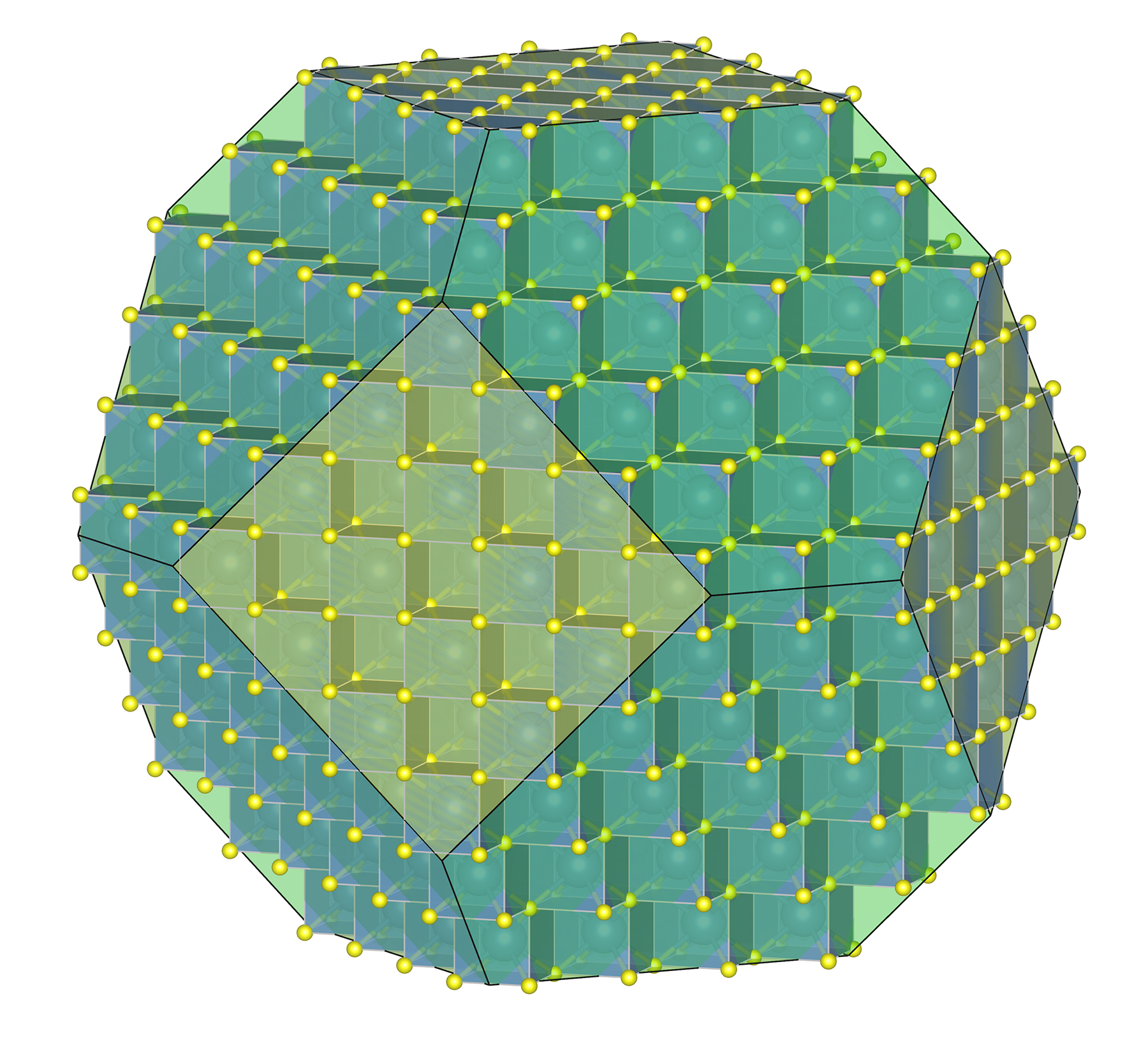
Figure 11.6 is the same figure we saw in Chapter 1. It shows the arrangement of atoms and building blocks in a fluorite crystal. Notice that the overall crystal has a sort of cube shape, and the building blocks are also cubes. This relationship between crystal symmetry and building block symmetry is at the heart of crystallography.
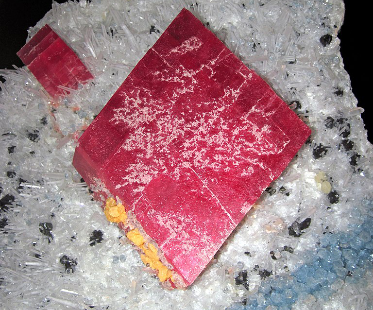
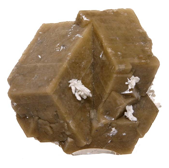
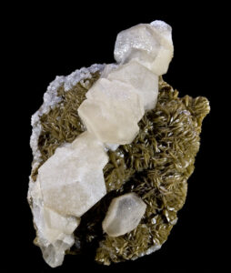
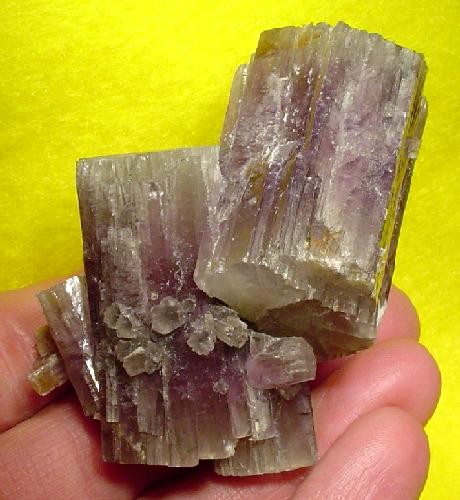
Early in the 1800s, several researchers found that crystals of similar, but not identical, chemical composition could have identical shapes. W. H. Wollaston (c. 1809) showed that calcite (CaCO3), magnesite (MgCO3), rhodochrosite (MnCO3), and siderite (FeCO3) all commonly formed the same distinctive rhombohedron-shaped crystals (Figures 11.7, 11.8, 11.9, and 11.10).
|
|
|
|
|
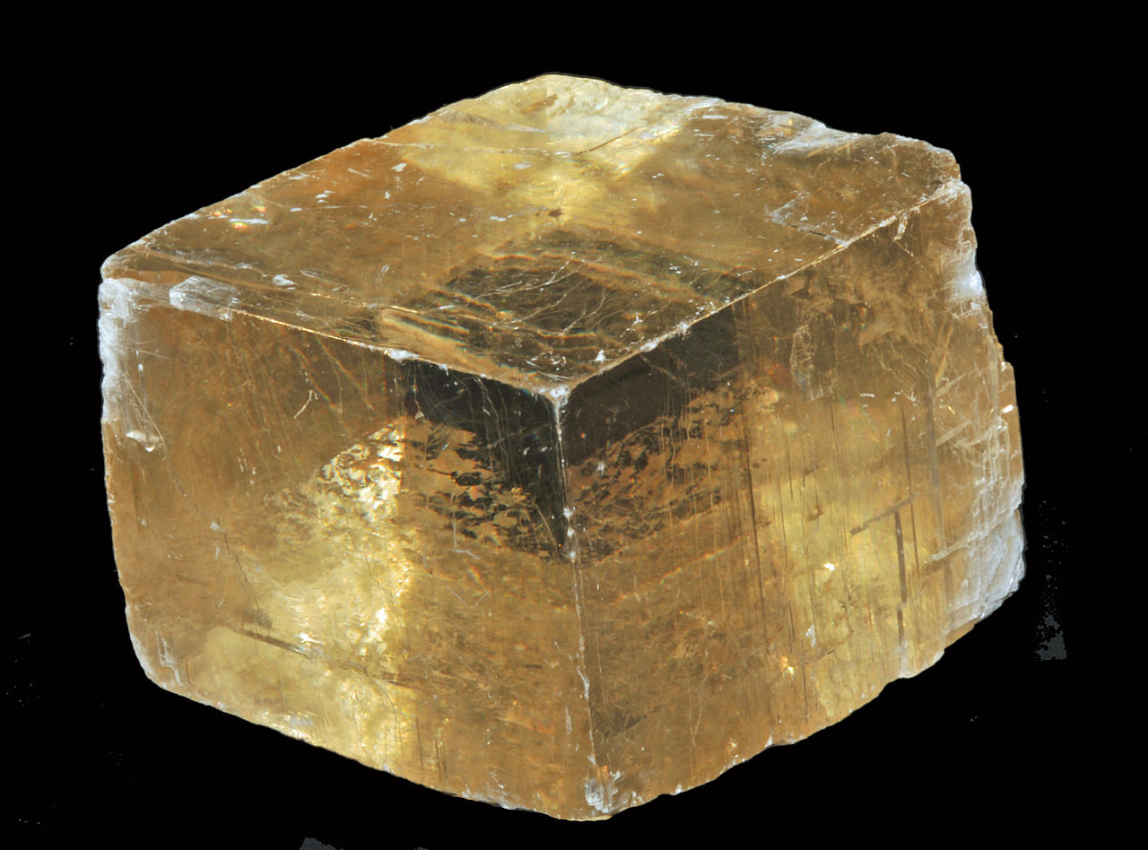
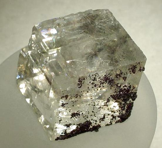
Those who studied sulfate compounds also found that crystals of different compositions had the same crystal shape. Both the rhombohedral carbonates and the sulfates are examples of isomorphous series. Wollaston and others concluded that when crystal shapes in such series are truly identical, the distribution of atoms within the crystals must be identical as well, even if the compositions are not. Minerals with identical atomic distributions are termed isostructural even if (unlike carbonates or sulfates) they have significantly different compositions.
Sometimes isostructural minerals form solid solutions because they can mix to form intermediate compositions. Fayalite (Fe2SiO4) and forsterite (Mg2SiO4) are isostructural and form a complete solid solution; olivines can have any composition between the two end members. In contrast, halite (NaCl) and periclase (MgO) are isostructural but do not form solid solutions. Calcite, magnesite, rhodochrosite, and siderite are isostructural but their mutual solubility is limited. They form only limited solid solutions, also called partial solid solutions.
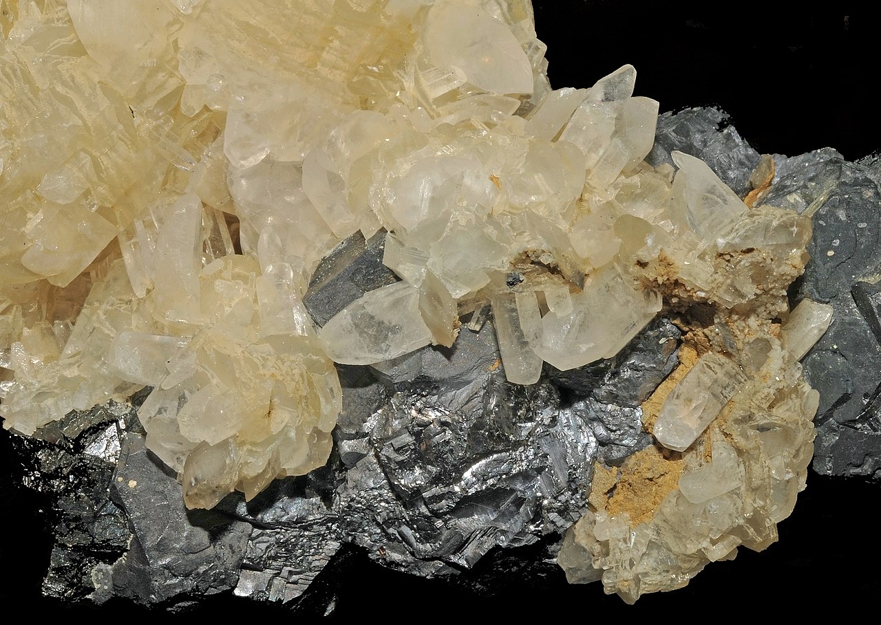
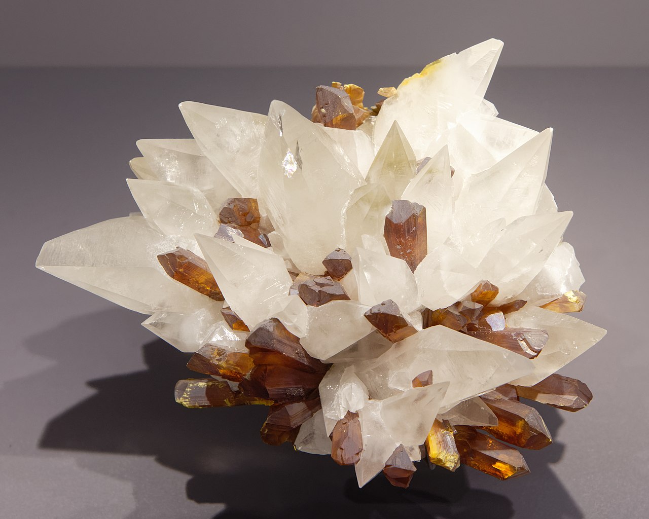
In 1821 Eilhard Mitscherlich, a student of Berzelius’s, discovered that the same elements may combine in different atomic structures. For instance, calcite and aragonite both have composition CaCO3, but they form different crystal shapes and have different physical properties. We call such minerals polymorphs because, although identical in composition, they have different atomic arrangements and crystal morphologies. Mineralogists have now studied several other CaCO3 polymorphs, but none except vaterite occur naturally. In calcite and vaterite the basic building blocks have rhomb-shaped faces, while in aragonite the faces are rectangles.
Figure 11.11 shows calcite and siderite crystals that do not have the same shapes as those above in Figures 11.7 and 11.10. Many minerals, especially carbonate minerals have multiple common habits. Figure 11.12 shows aragonite crystals and Figure 11.13 shows vaterite crystals. Both minerals, like calcite, have composition CaCO3.
By the early/mid 1800s it was clear that there was no direct correlation between the shapes of building blocks and crystal composition, as Haüy had originally thought. Despite flaws in some of his ideas, however, we must credit René Haüy as one of the founders of crystallography. In later years, he pioneered the application of mathematical concepts to crystal properties, which established the basis for modern crystallography, and crystallographers still use much of his work today. We now accept that:
• All crystals have basic building blocks called unit cells.
• The unit cells are arranged in a pattern described by points in a lattice.
• The relative proportions of elements in a unit cell are given by the chemical formula of a mineral.
• Crystals belong to one of seven crystal systems.
• Unit cells of distinct shape and symmetry characterize each crystal system.
• Total crystal symmetry depends on both unit cell symmetry and lattice symmetry.
We can define unit cells in multiple ways for any mineral structure. In general we choose the cell that is the smallest possible unit that reflects both the composition and symmetry of a mineral. Most unit cells contain less than 10 to a few dozen atoms. The atoms may be entirely with the cell, on cell edges or faces, or at the corners.
11.2 Translational Symmetry
In the previous chapter we discussed symmetry due to rotation, reflection, and inversion. These are all types of point symmetry. The orderly repetition of patterns due to translation is another form of symmetry, called space symmetry. Space symmetry differs from point symmetry.
Space symmetry repeats something an infinite number of times to fill space, while point symmetry repeats something a discrete number of times and only describes symmetry localized about a central point. Point symmetry operators return a dot or a crystal face to its original position and orientation after 1, 2, 3, 4, or 6 repeats of the operation, but space symmetry operators do not. Translation goes on (almost) forever!
We often envision translational symmetry by thinking about a lattice, a set of an infinite number of points related by translations. In two dimensions, a lattice is called a plane lattice. In three dimensions, a lattice is a space lattice. Whether two or three dimensional, lattices are imaginary – they are not physical entities – they are patterns that we use to describe translational symmetry.
Figure 11.14a shows an example of how we depict a plane lattice. The vectors t1 and t2 are translation operators that generate the entire lattice from a single starting point. This drawing only shows part of the lattice; in your mind you should picture it extending infinitely in all directions.
Translational symmetry, like all symmetry, is a property that objects may have. If we have an object or a drawing, we can describe its translational symmetry. But it does not work the other way around because many different objects or drawings may have identical symmetry.
For example, Figure 11.14b (above) shows cats related by the same symmetry depicted in Figure 11.14a. Figure 11.14c shows parallelograms related by the same symmetry. And Figure 11.14d shows colored circles (that might represent atoms) related by the same symmetry.
The four drawings in Figure 11.14 have more than just translational symmetry. They also contain multiple 2-fold rotation axes perpendicular to the plane of the page. And there are inversion centers, too. So we see that translational symmetry can combine with other kinds of symmetry.
Repetitive patterns are composed of motifs, which are designs that repeat, such as a flower pattern that might be on wallpaper. The term motif is used in an analogous way in music to refer to a sequence of notes that repeat. Interior decorators or clothing designers use the term to describe a common theme or element in their work.
A motif (whether it comprises two cats, a parallelogram, or colored circles) and empty space around it, make up unit cells that repeat to create an infinite pattern. The lattice describes the nature of the repetition, with each lattice point representing one motif. But lattice points do not correspond to any particular point on a motif. We could choose them at the motif’s center or one of its corners and the result would be the same.
Figure 11.15 shows unit cells that can be used to generate the patterns seen in Figure 11.14. These unit cells are parallelograms with dimensions and angles that match the translation vectors of the lattice. Notice that each one of these unit cells has a 2-fold axis of symmetry perpendicular to the page and an inversion center. This symmetry must be present to be consistent with the lattice.
11.3 Unit Cells and Lattices in Two Dimension
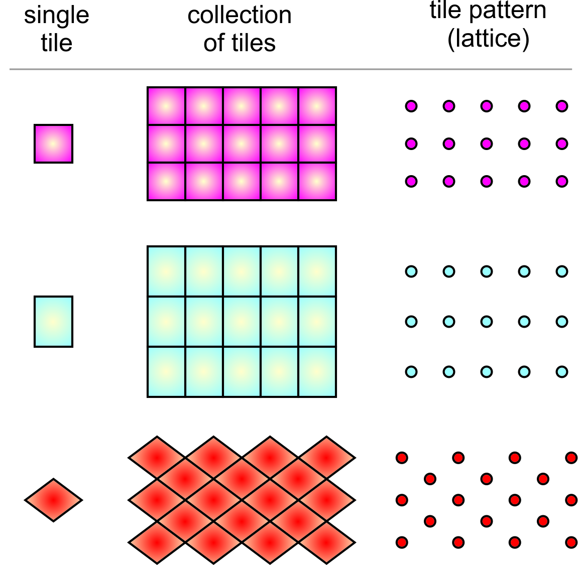
What possible shapes can unit cells have? Mineralogists begin answering this by considering only two dimensions. This is much like imagining what shapes we can use to tile a floor without leaving gaps between tiles. Figure 11.16 shows some possible tile shapes. In the right-hand column of this figure, a single dot has replaced each tile to show the plane lattice that describes how the tiles repeat. This figure does not show all possible shapes for tiles or unit cells, but as we will see later the number of distinct possibilities is quite small.
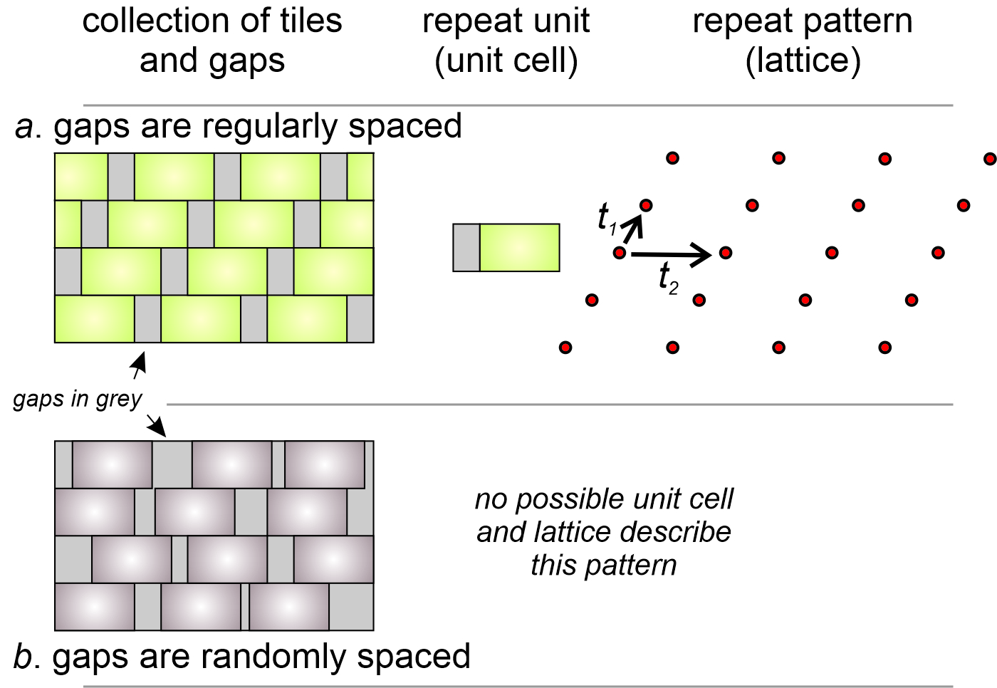
What happens when gaps occur between tiles? Figure 11.17 shows the two possibilities: the gaps may be either regularly (11.17a) or randomly (11.17b) distributed. If regularly distributed, we can define a unit cell that includes the gap, as we have in drawing 11.17a. The two vectors, t1 and t2 and the lattice they create describe how the unit cell repeats to make the entire tile pattern.
If gaps between tiles are random, the entire structure is not composed of identical building blocks that fit together in a regular way. It is not repetitive and we cannot describe it with a unit cell and a lattice. It does not, therefore, represent the symmetry of a possible crystal structure and we need not consider it further.
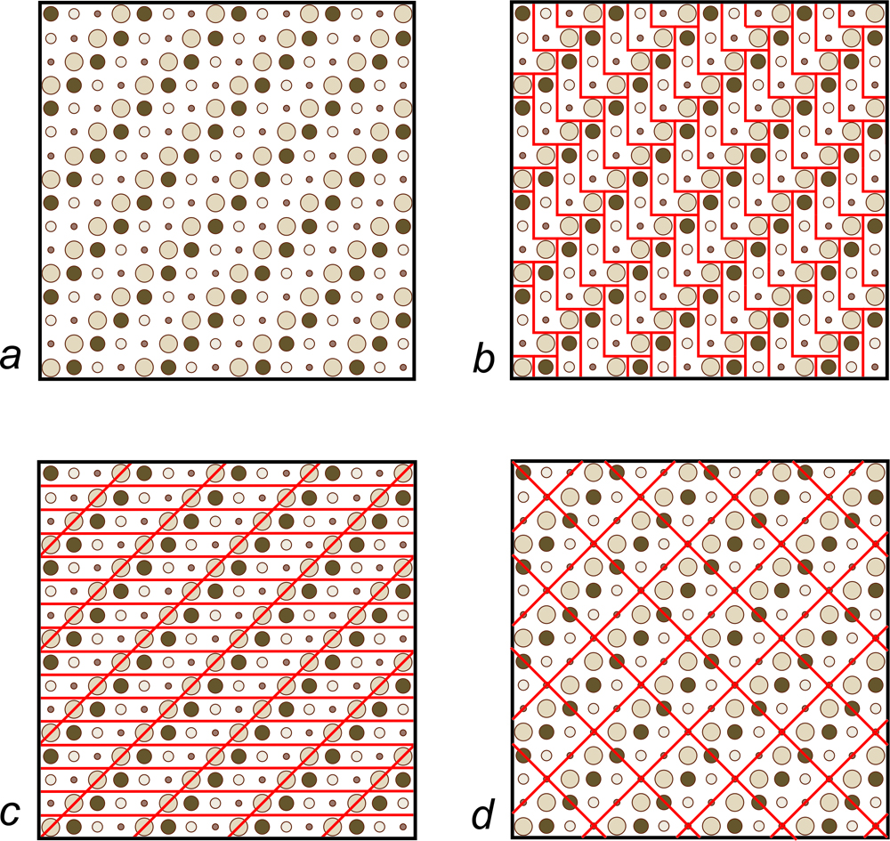
Various complex patterns can appear on tiled floors, but the tiles are usually simple shapes such as squares or rectangles. For example, suppose we wish to tile a floor in the pattern shown in Figure 11.18a. We could use L-shaped tiles, shown in red in Figure 11.18b. However, parallelogram- or square-shaped tiles would get us the same pattern (Figures 11.18c and d). Other shapes, too, would work.
We can make any repetitive two-dimensional pattern, no matter how complicated, with tiles of one of four fundamental shapes: parallelogram, rhomb (a parallelogram with sides of equal length), rectangle, and square. These shapes are relatively simple compared to more complex ones we could choose, and they reveal symmetry that is present. So, they are used by mineralogists and preferred by tile makers.
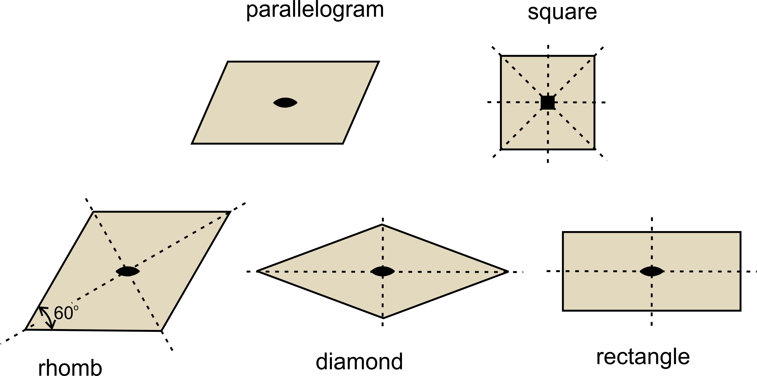
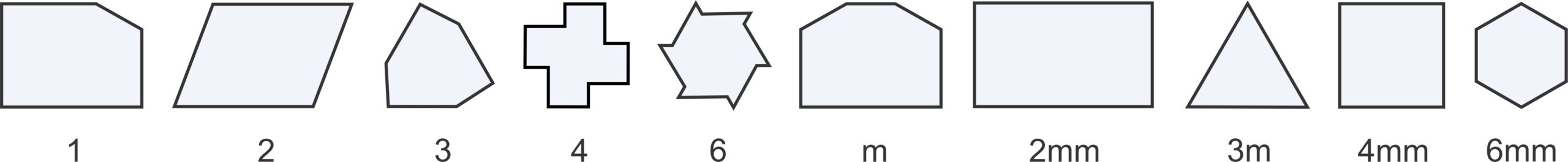
For reasons we will see later, we usually distinguish two types of rhombs (parallelograms with sides of equal length): those with nonspecial angles between sides and those with 60o and 120o angles between sides. For the rest of this chapter, we will refer to the general type of rhomb as a diamond, and the term rhomb will be reserved for shapes with only 60o and 120o angles (and sides of equal length). So, Figure 11.19 shows the five basic shapes, the only ones needed to discuss two-dimensional unit cells, and their symmetries.
We can now explain why we only considered 1-, 2-, 3-, 4-, and 6-fold rotational symmetry in the previous chapter. Two-dimensional shapes with a 5-fold axes of symmetry, for example, cannot be unit cells because they cannot fit together without gaps. We can verify this by drawing equal-sided pentagons on a piece of paper. No matter how we fit them together, space will always be left over. The same holds true for equal-sided polyhedra with seven or more faces. They cannot fit together to tile a floor. And if the shapes cannot fit together in two dimensions, they cannot fit together in three dimensions.
11.3.1 Motifs and Unit Cells
We can think of atomic arrangements as starting with one motif. The motif is then reproduced by translating (moving) it a certain distance and reproducing it. The distance of the translation is the distance between lattice points. If a dot replaces each motif, we get the lattice.
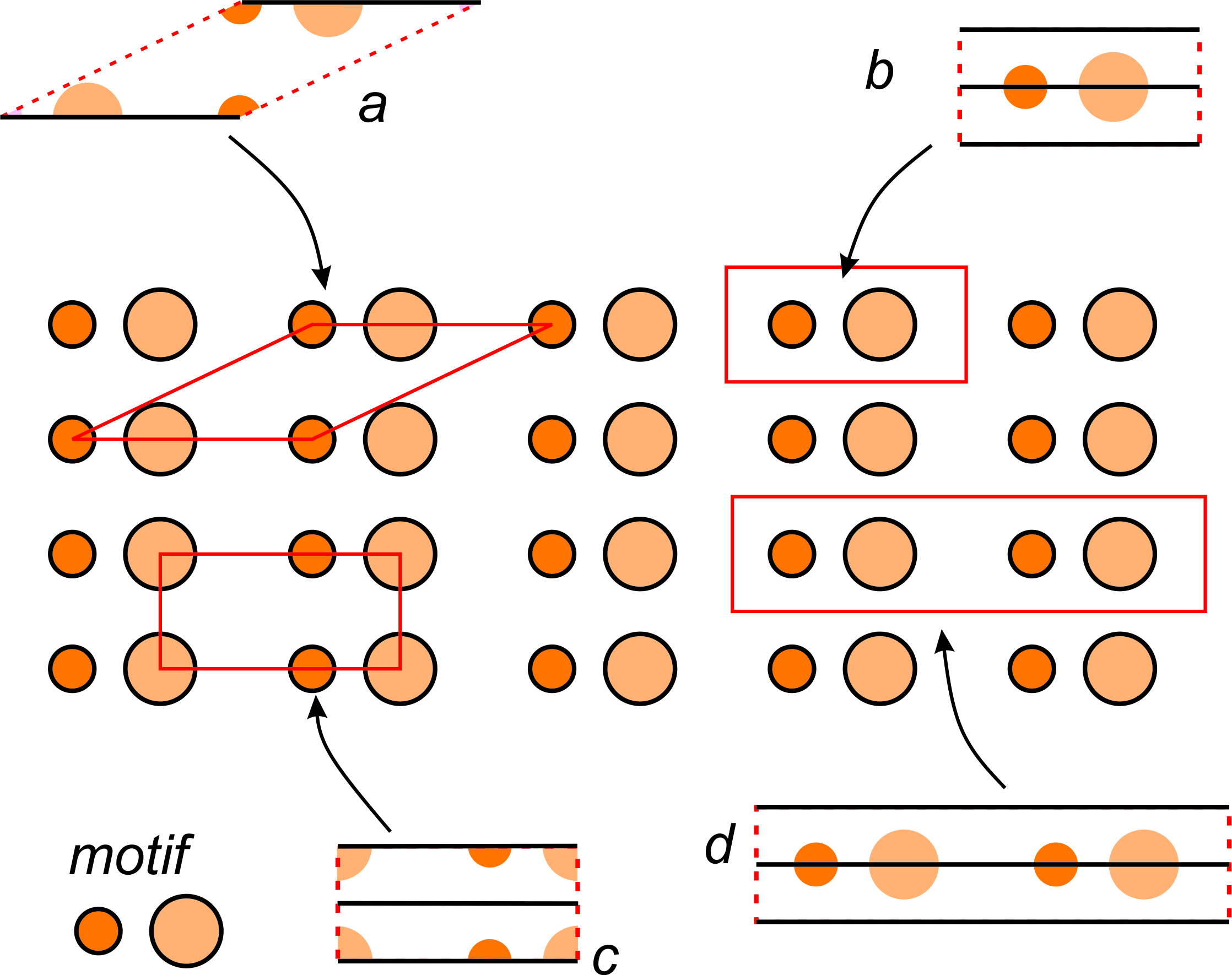
Figure 11.20 shows a pattern made of two atoms, symbolized by different sized orange circles. The entire pattern consists of motifs composed of one of each kind of atom. The pattern contains multiple horizontal mirror planes but no other symmetry.
The figure shows several possible choices of unit cells (labeled a through d). In the individual unit cell drawings, solid black lines show mirror planes of symmetry.
Unit cells a, b, and c contain only one motif in total (one small orange circle and one larger lighter orange circle). We call them primitive because they are the smallest unit cell choices possible. All primitive unit cells contain exactly one motif, but atoms within a primitive unit cell may be in parts as in unit cell c. Add up the parts and you get one motif. We term unit cell d doubly primitive because it contains two motifs. Triply primitive unit cells contain three motifs, etc.
We can always choose a primitive unit cell for a repetitive pattern of atoms, but sometimes a primitive cell does not show symmetry clearly. By convention, we usually choose the smallest unit cell that contains the same symmetry as the entire pattern or structure. In Figure 11.20, unit cell b would be the choice of most crystallographers because it is simple, primitive, does not contain any partial atoms, and contains a horizontal mirror plane (which is the same symmetry as the entire pattern). Note that unit cell a, while also being primitive, does not have a mirror plane of symmetry within it; the other choices do.
|
|
|
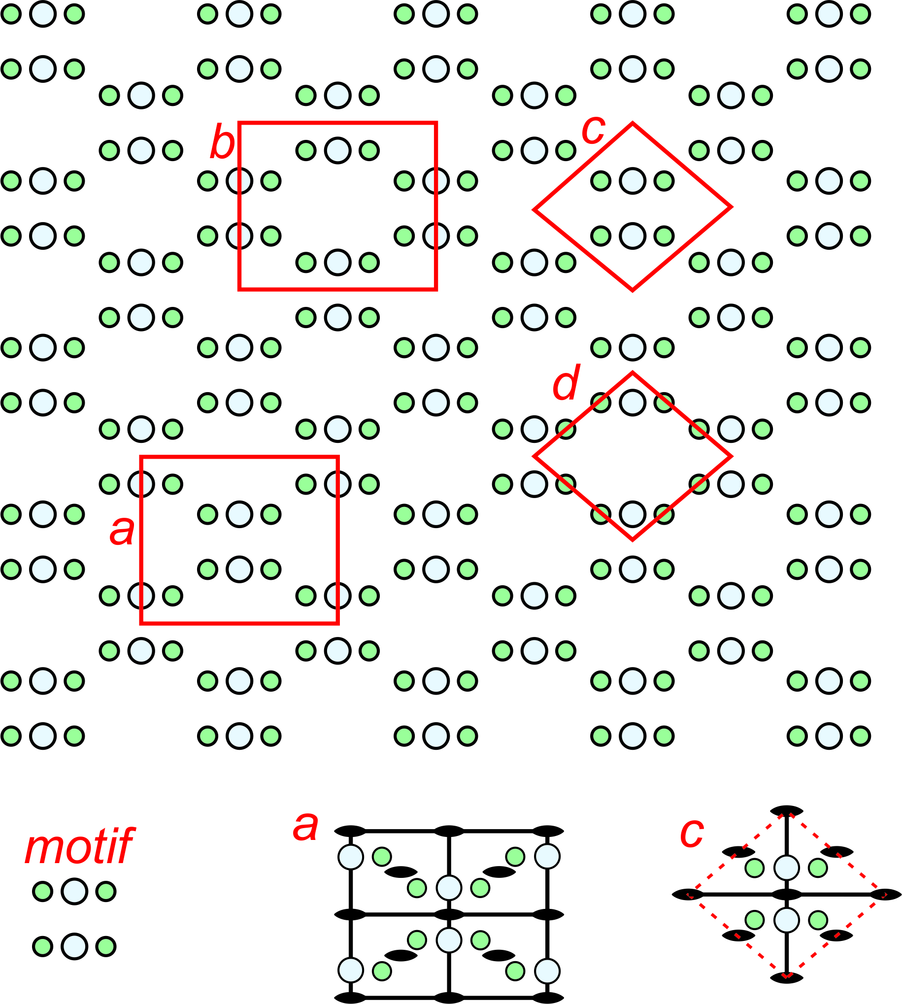
The pattern shown in Figure 11.20 has relatively simple symmetry; the patterns in Figures 11.21 and 11.22 have more. Figure 11.21 shows an orthogonal (containing lots of 90o angles) arrangement of atoms. The repeating motif contains six atoms – four green and two larger light blue ones. The letters a, b, c, and d designate four possible choices for unit cell. Cells c and d are primitive, containing six atoms total, although some are on the edges in cell d so only half of each green atom is in the unit cell. Cells a and b are doubly primitive but they are rectangular shapes. The symmetries of two of the unit cells are shown in the bottom of the figure. Solid black lines designate mirrors and lens shapes designate 2-fold axes. Unit cell a, although being double primitive, is the one that best shows the symmetry elements and so would be the choice of most crystallographers.
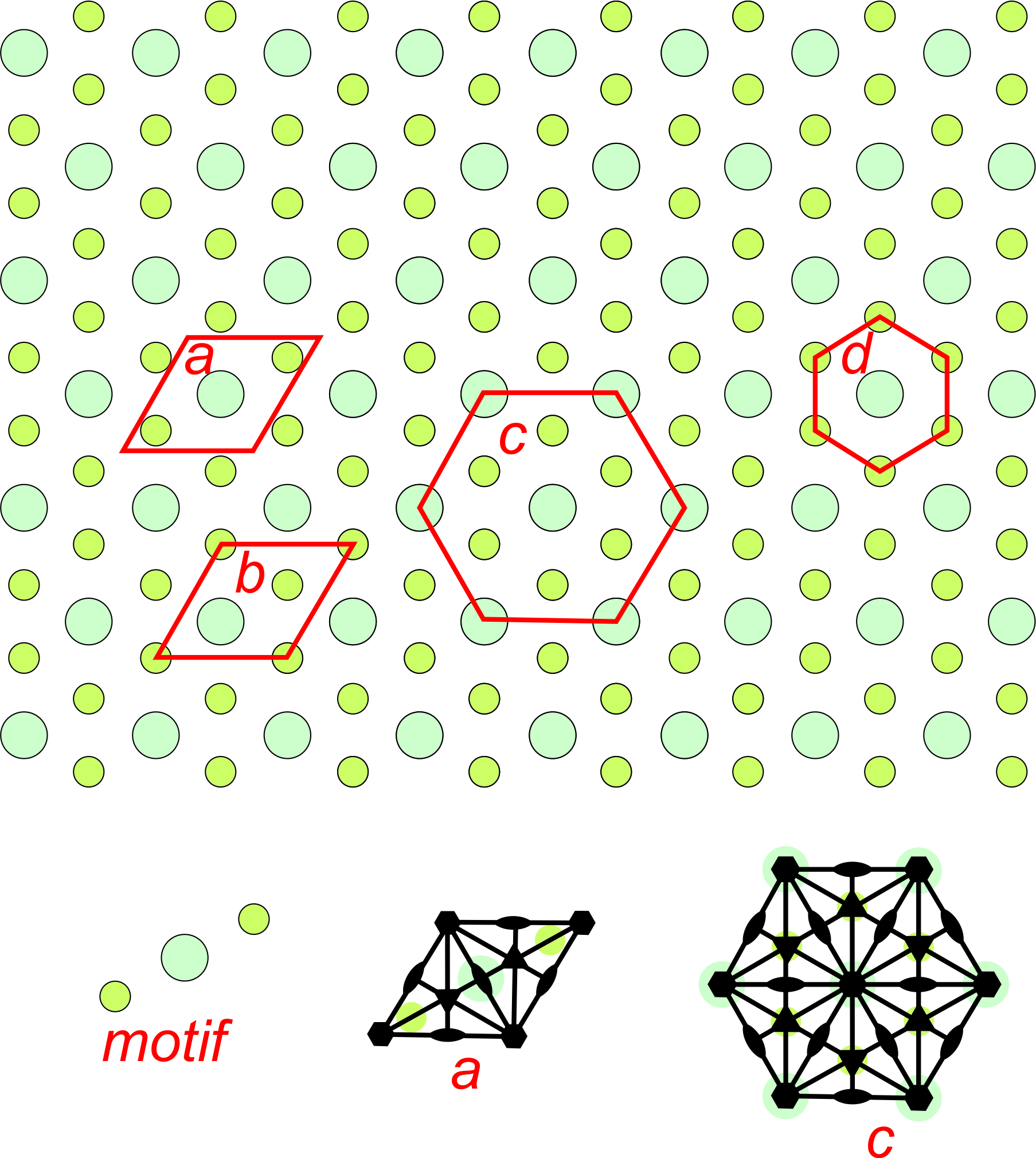
Figure 11.22 shows an overall hexagonal pattern. The motif consists of one large turquoise atom and two smaller green atoms. Four possible choices for unit cells are shown. Drawings in the bottom of the figure show symmetry of two of the potential unit cell with solid black lines as mirrors, lens shapes as 2-fold axes, and hexagons as 6-fold axes. Two of the potential unit cells are rhomb shaped and two are hexagonal. Because the overall pattern has hexagonal symmetry, unit cells c and d are preferred choices compared with the other two. Unit cell d is primitive, but does not include all the symmetry. (It does not have 2-fold rotation axes.). So cell c is the best choice. This pattern demonstrates why we treat rhombs with 60̊o and 120̊o angles at their corners as special cases – they sometimes result in hexagonal symmetry while diamonds with general angles at their corners cannot.
Although crystallographers follow standard conventions, they are often forced to make choices. If they choose primitive unit cells, each lattice point corresponds to one unit cell and one motif. If they choose nonprimitive unit cells, lattices represent the way motifs repeat, but not the way unit cells repeat because there is more than one lattice point per unit cell.
11.3.2 What are the Possible Plane Lattices?
Above we looked at a number of different examples of lattices and unit cells. To get a complete list of possibilities let’s look at all the possible plane lattices. In a plane lattice, lattice points are related by two vectors describing translation. The vectors may be orthogonal (perpendicular to each other) or not. And they may be equal length or not.
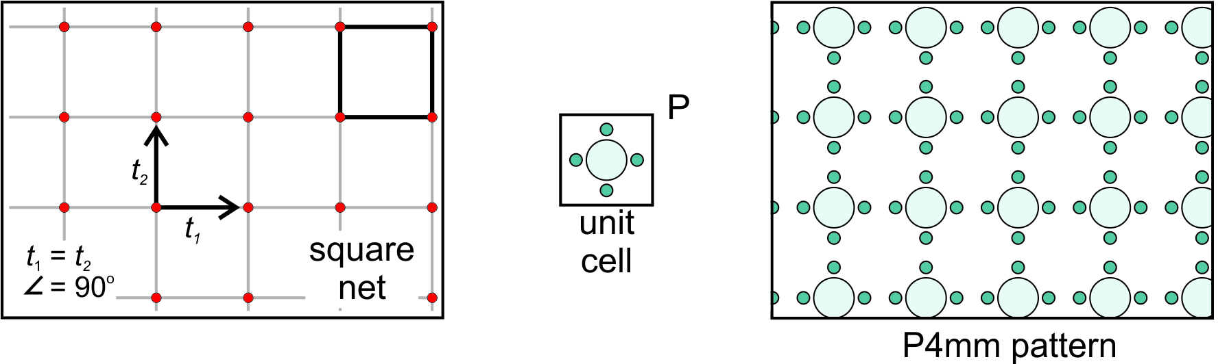
Square Net: Let’s consider the simplest possibility – that the vectors are orthogonal and of equal length. This produces a square net (lattice), as shown on the left in Figure 11.23, below. If we choose a square unit cell and put a motif (five atoms) with square symmetry within it, we get the pattern seen in the drawing on the right. This pattern has the same symmetry as the lattice and of the unit cell. The symmetry includes 4-fold and 2-fold rotation axes, and mirror planes that intersect at 45o and 90o. The P next to the unit cell reminds us that it is primitive. Because the overall atomic arrangement contains a 4-fold axis and two differently oriented mirrors (ones that are perpendicular to the faces of the unit cell, and ones that follows the diagonal of the unit cell), we describe its symmetry as P4mm.
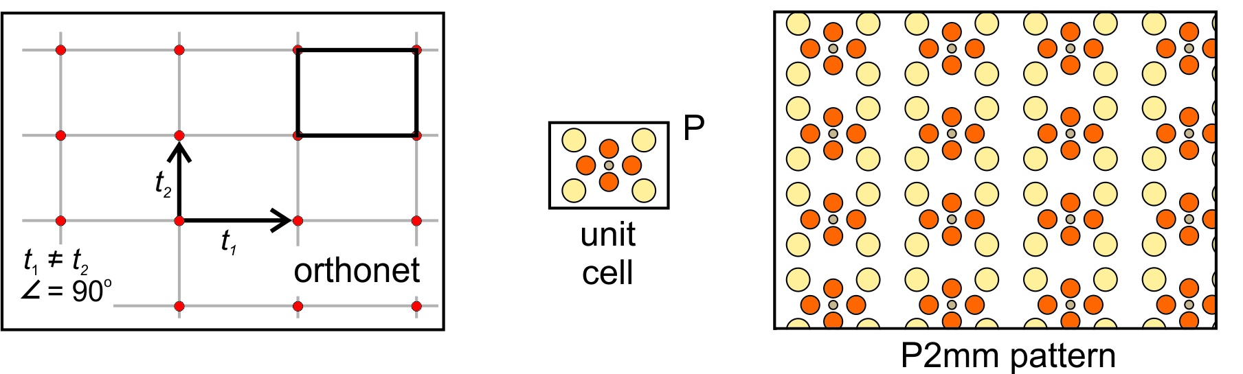
Orthonet: Suppose the two vectors relating lattice points are orthogonal but not of equal length. If so, we get an orthonet, equivalent to a rectangular lattice. Figure 11.24, below, shows an example. We can choose a rectangular unit cell and add a rectangular motif that contains nine atoms. We get the pattern shown on the right in Figure 11.24. Note that the lattice, the primitive (P) unit cell, and the pattern have equivalent symmetry that includes mirror planes and 2-fold rotation axes. The overall atomic arrangement contains a 2-fold axes with horizontal and vertical mirrors; we describe its symmetry as P2mm.
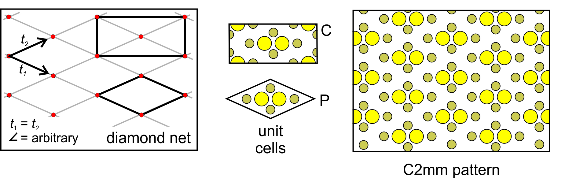
Diamond Net: A third general possibility is that the vectors relating lattice points are of equal magnitude but intersect at a non-special angle. This combination produce a diamond net (lattice) like the one below in Figure 11.25. We can add a motif of six atoms to a diamond-shaped unit cell to get the atomic arrangement shown on the right in Figure 11.25. But, notice that we can also choose a rectangular unit cell that is doubly primitive – it has an extra lattice point at its center and contains two motifs. Either unit cell will generate the same pattern. We use the letter P to indicate the primitive unit cell, and the letter C to indicate the cell with an extra lattice point in its center. The rectangular unit cell shows the vertical and horizontal perpendicular mirror planes and the 2-fold rotation axes more clearly than the diamond shaped one. So, we describe the symmetry of the pattern as C2mm.
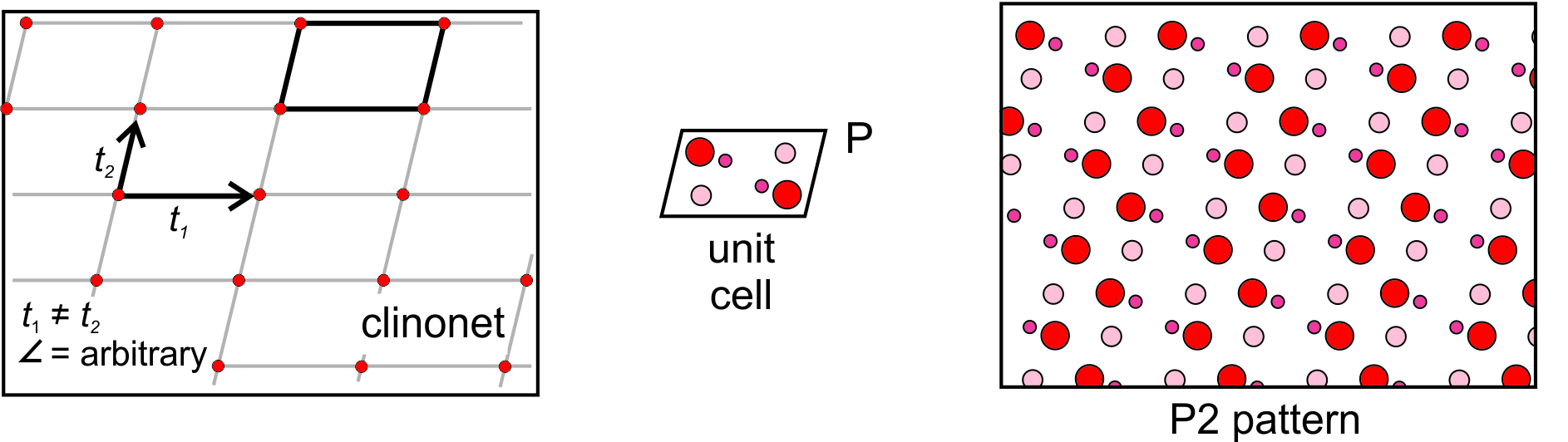
Clinonet: The fourth possibility is that the two translation vectors are of different lengths and are not orthogonal. This produces a clinonet (Figure 11.26) that corresponds to a primitive unit cell with the shape of a parallelogram. Adding a motif containing six atoms gives us the atomic arrangement on the right in Figure 11.26. There are no mirror planes here – the only symmetry is 2-fold rotation perpendicular to the page. The arrangement of atoms has symmetry P2.
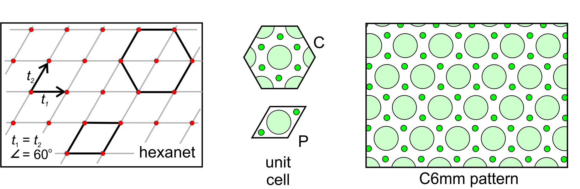
Hexanet: The fifth possible net is the created by the special case when the two translation vectors are of equal magnitude and intersect at 60o. This combination gives us a hexanet (hexagonal lattice) like the one shown in Figure 11.27, below. As with the diamond net, we can choose either a primitive rhomb-shaped unit cell or a triply-primitive hexagonal unit cell. The lattice and the overall atomic arrangement have hexagonal symmetry, so the hexagonal unit cell (which also has hexagonal symmetry) is generally chosen. A 6-fold axis and two kinds of mirrors at different orientations characterize this pattern. One set of mirrors is perpendicular to the faces of the hexagonal unit cell; the other passes through the corners of the unit cell. We designate the overall symmetry as C6mm.
11.3.3 How May Motifs and Lattices Combine?
Above, we saw examples where the lattice, the motif, and the overall pattern had the same symmetry. This was true in Figures 11.23, 11.24, 11.25, and 11.26. But, it was not true in Figure 11.27 where the motif and a primitive unit cell (labeled P) consisted of 3 atoms and a mirror plane of symmetry, while the lattice and overall pattern have hexagonal symmetry. Notice that in Figure 11.27, we could choose a hexagon-shaped triply primitive unit cell (labeled C) that had the same symmetry as the lattice and overall pattern. Because the triply primitive cell shows the 6-fold symmetry, it is the best choice.
This leads to an important second law of crystallography:
blank■ If a motif has certain symmetry, the lattice must have at least that much symmetry.
A motif with a 4-fold axis of symmetry requires a square plane lattice because it is the only plane lattice with a 4-fold axis. A motif, however, may have less symmetry than a lattice. If a motif has a 2-fold axis of symmetry, it may be repeated according to any of the five plane lattices because they all have 2-fold axes of symmetry.
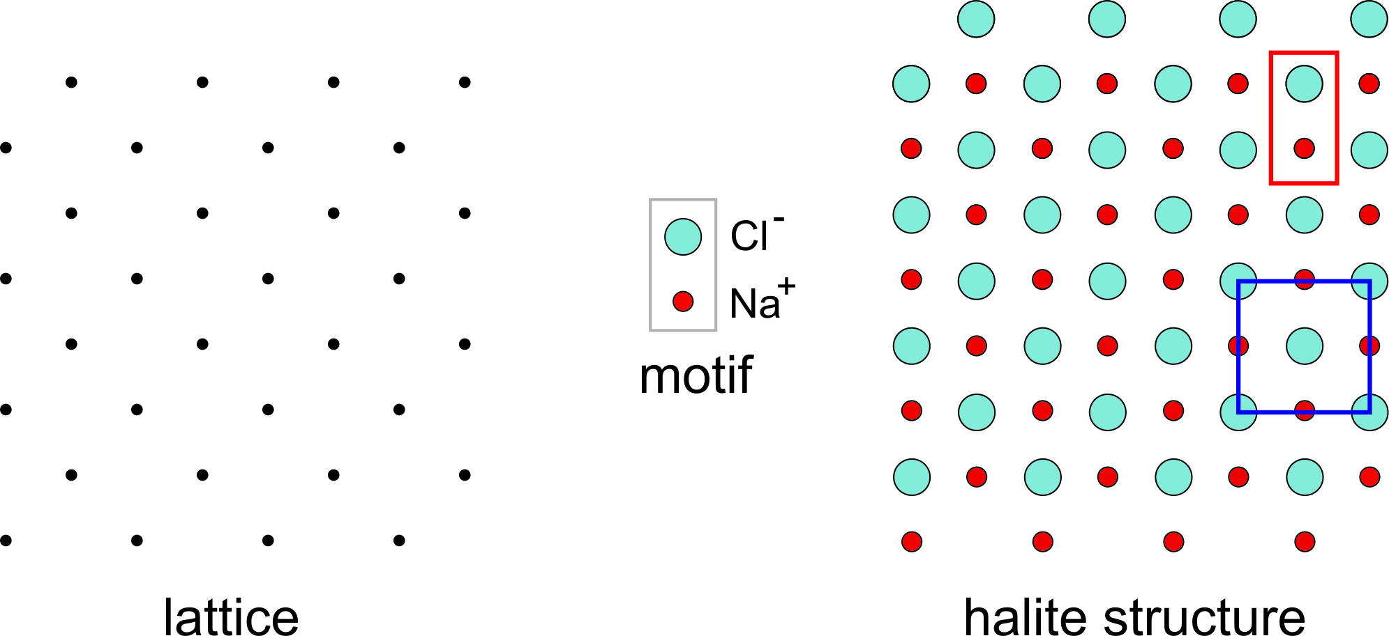
Halite (NaCl) is an excellent example of a mineral in which the simplest motif has less symmetry than the lattice. Figure 11.28 shows a two-dimensional model of the atomic arrangement in halite. The lattice is on the left and the motif, consisting of a Cl– anion and an Na+ cation is shown in the center of the figure.
In two dimensions the lattice has square symmetry (although it is tilted to 45o in this drawing), but the motif, consisting of one Na and one Cl atom, does not. Putting a motif at every lattice point gives the atomic arrangement on the right. A primitive unit cell (P), containing two atoms (outlined in red), is rectangular and does not have square symmetry. Notice, however, that we can choose a nonprimitive unit cell containing four atoms and two motifs (outlined in blue) that has square symmetry. This would not be possible if the lattice did not have “at least as much symmetry as the motif.”
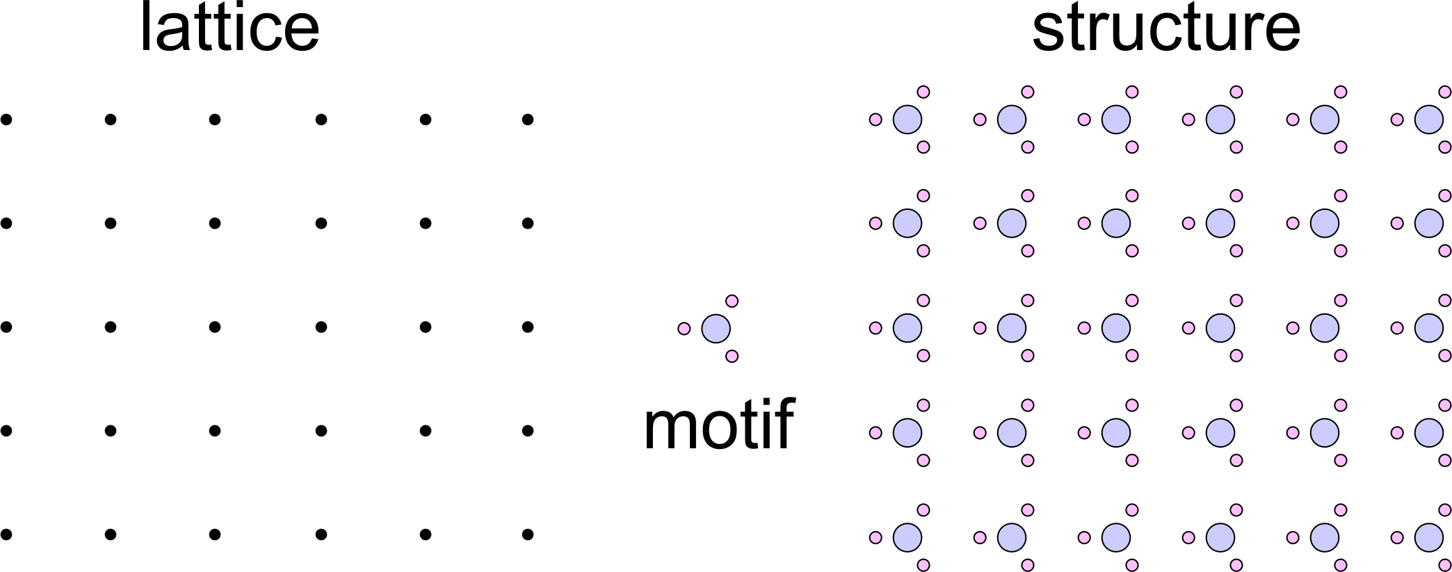
Figure 11.29 shows an impossible combination of a lattice and a motif. The lattice has 4-fold rotational symmetry, the motif has 3- fold symmetry. But the combination yields a structure that has no rotational symmetry. Looking at this figure should give you the sense that something is wrong. And, it is. If the motif really has 3-fold symmetry, it is identical in three directions 120o apart. So bonds around it should be the same in three directions 120o apart. But, they are not in the structure drawing. A motif with 3-fold symmetry requires a lattice that has at least 3-fold symmetry. There is only one and it is a hexanet. The lattice cannot be a square lattice.
11.3.4 Glide Planes of Symmetry
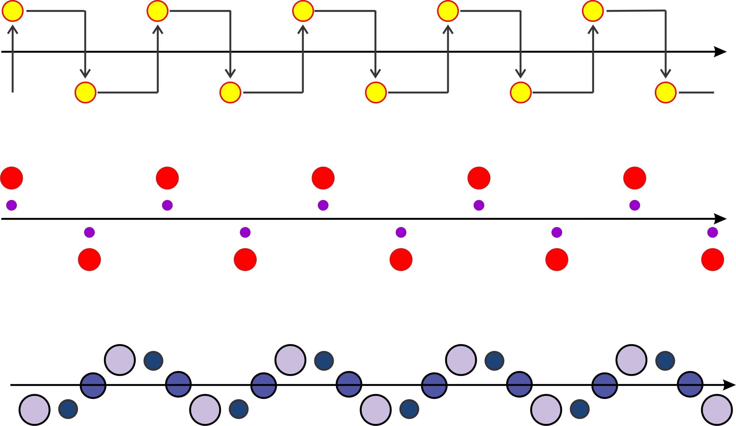
Previously, we have looked at point symmetry that included rotation, reflection, inversion, and translation. If we combine translation and reflection (mirror planes) we find there is one other kind of symmetry that may be present in two-dimensional atomic arrangements: glide planes. Figure 11.30 shows three examples of a motif repeating by a glide plane. Glide planes are combinations of translation and reflection, in much the same way that rotoinversion axes are combinations of rotation and inversion. Thus, in Figure 11.30, a motif (a yellow atom, two red atoms, or three blue/purple atoms in these examples) is translated before being reflected across the plane.
Glide planes are a kind of space symmetry that continues indefinitely. They are only one kind of symmetry operator that combines translation with elements of point symmetry. Screw axes a related operator that combines translation with rotation, do not exist in two dimensions. We will talk about both glide planes and screw axes in more detail later when we return to three dimensions and discuss space groups. For now it is sufficient to know that glide planes exist.
11.3.5 Plane Groups
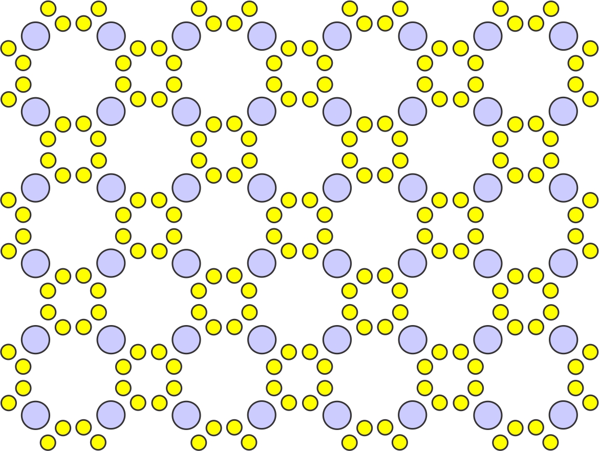
So, motifs and lattices combine to produce repetitive patterns. In two dimensions, atomic motifs may have 1-fold, 2-fold, 3-fold, 4-fold, or 6-fold symmetry. And they may or may not contain mirror planes of symmetry; this gives 10 distinct point symmetries. Lattices may be square nets, orthonets, diamond nets, clinonets, or hexanets – five choices. And atomic arrangements may include glide planes. If all combinations were possible, we would have many possibilities. But there are constraints. For example, as we saw above, if a motif has certain symmetry, the lattice must have at least that much symmetry. There are other constraints, too. A square net, for example, can only combine with motifs that have 4-fold symmetry. And some combinations of symmetry and lattice require other symmetry to be present too. In all, there are only 17 possible symmetries that a 2D atomic arrangement can have. These are the 17 plane symmetry groups, also called plane groups, plane crystallographic groups, or wallpaper groups (because they describe how patterns may repeat in wallpaper).
The drawings in Figure 11.31 depict unit cells for the 17 plane groups. Geometric symbols show rotation axes, solid red lines are mirror planes, and blue dashed lines are glide planes. The labels under each unit cell are the standard abbreviations used by crystallographers. These labels do not include all symmetry – several of the groups contain 2-fold axes or glide planes not in the abbreviations – but the additional symmetry must be present.
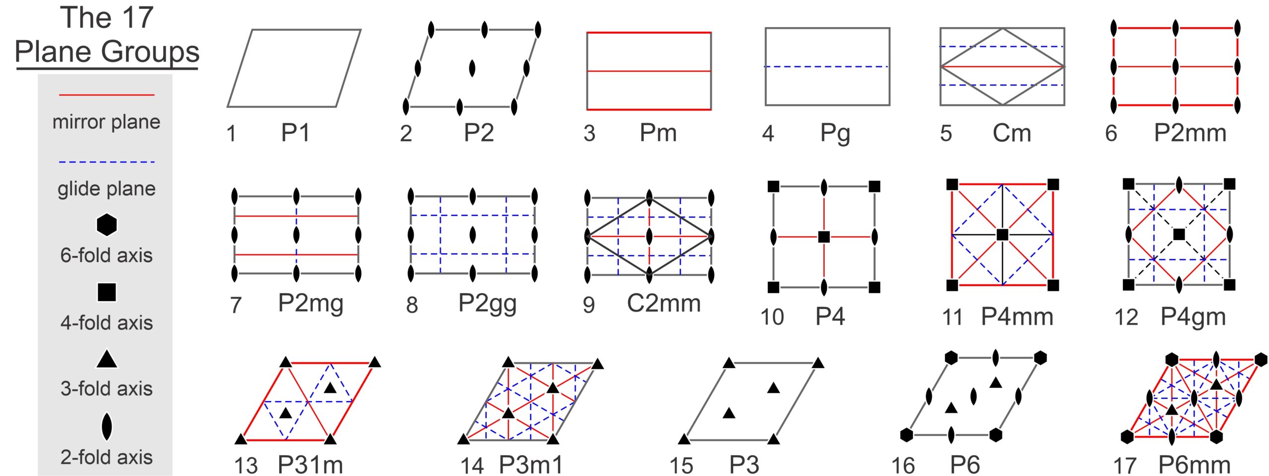
Three of the 17 possibilities involve square unit cells, seven involve rectangular unit cells. Of those seven, two (Cm and C2mm) are centered cells and the overall pattern could be made with a primitive diamond-shaped unit cell (also shown) instead of a doubly primitive rectangular unit cell. Refer to the discussion of diamond nets earlier in this chapter. By convention, we generally describe these plane groups using the centered cell, but it really makes little difference.
Two of the symmetry groups have unit cells shaped like a parallelogram, and the five across the bottom of the diagram have rhomb-shaped unit cells. The rhomboid cells could be combined to produce non-primitive hexagon-shaped cells. Refer to the discussion of hexanets earlier in this chapter. Some of the rhomb-based symmetry groups (the bottom two on the right) have 6-fold symmetry and some do not, but the distinction is hard to see. The examples below in Box 11-1 will make this more clear.
Box 11-1 The 17 Plane Symmetry GroupsIn two dimensions, atomic arrangements may have one of 17 possible symmetries. Figure 11.32 (below) contains examples of each. The examples include larger patterns with individual unit cells below. The unit cells use standard symbols to show the locations of rotation axes, mirror planes, and glide planes. We have included both diamond-shaped and rectangular unit cells for the two centered groups (Cm and C2mm). And, for the rhomb-shaped cells, a larger hexagonal (non-primitive) cell is shown that helps make the distinction between those with 3-fold and 6-fold symmetry (although you may have to look at the pdf version and enlarge this figure to see the details). In the labels: 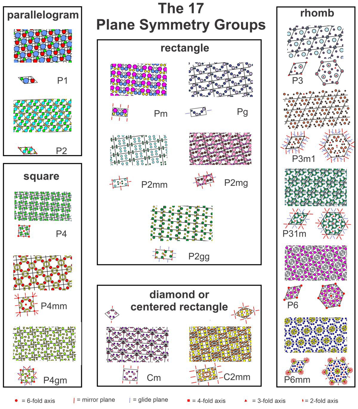 For a larger version of the figure above, use this link to open a pdf version. |
11.4 Unit Cells and Lattices in Three Dimensions
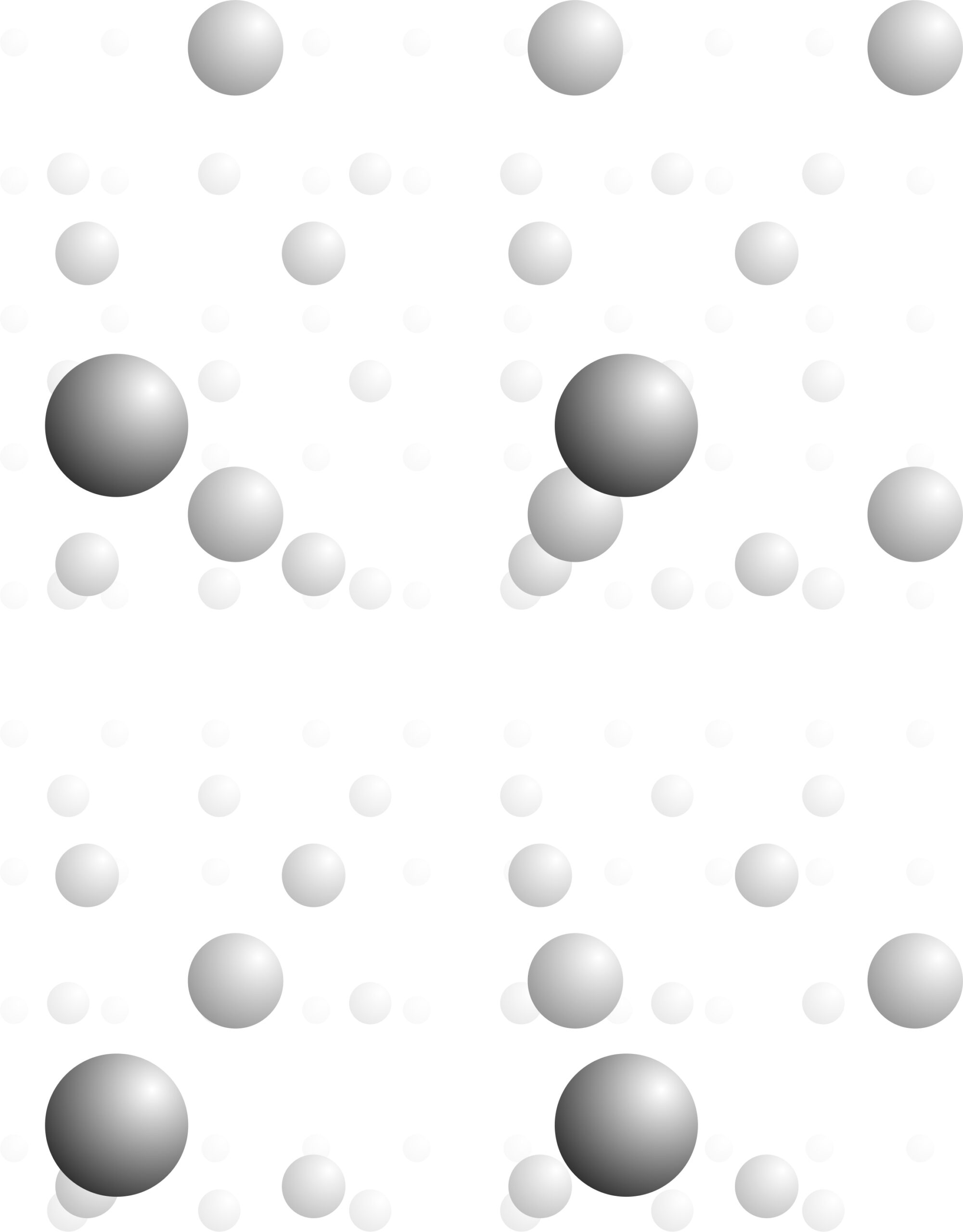
In two dimensions, patterns are made of unit cells, and lattices describe how unit cells and motifs repeat. These relationships are the same in three dimensions. Figure 11.33, for example, shows a single atom repeated an indefinite number of times and disappearing into the distance. Choose any four nearest neighbor atoms and you can connect them to get a 3D unit cell that is the basis for the entire atomic array.
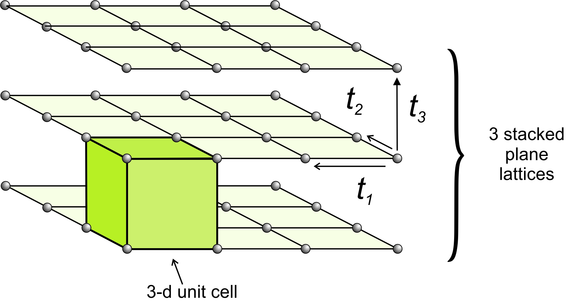
In two dimensions, two vectors describe the translation that relates lattice points. To move from two dimensions (planes) to three dimensions (space), we need only to define a third vector, t3, that translates a plane lattice some distance where it is repeated. We continue this process many times to get a space lattice. Figure 11.34 shows an example.
We can start with any of the two-dimensional plane lattices. The third translation may be orthogonal to one or both of the first two translations, but it need not be. Its magnitude may be the same as one or both of the first two translations, or not. We can envision space lattices as identical points that repeat indefinitely in three-dimensional space.
(Note that, for convenience, in this and subsequent drawings, we are choosing unit cells with lattice points at their corners. But we could choose unit cells with lattice points at their centers or anywhere else in the cell, because lattice points are simply patterns showing how unit cells repeat. It makes no difference if the lattice point corresponds to the corner, center, or any other point in the motif.)
In Figure 11.33, we start with a square lattice, and choose a third translation vector (t3) that is equal in magnitude and also perpendicular to the first two. The result is in an overall cubic lattice. Connecting eight nearest-neighbor lattice points gives us a cubic unit cell. The plane lattices had symmetry 4mm; the cubic unit cell has symmetry 4/m32/m (described in the previous chapter).
If we stack a square net directly above another square net, as in Figure 11.33, the 4-fold rotation axis and the mirror planes line up and we preserve all symmetry. But, suppose the third translation is not perpendicular to the first two, and each square net is slightly offset from the ones above and below it. If so, rotation axes and mirrors in the different nets will not line up. The resulting space lattice may contain no 4-fold axes and no mirrors.
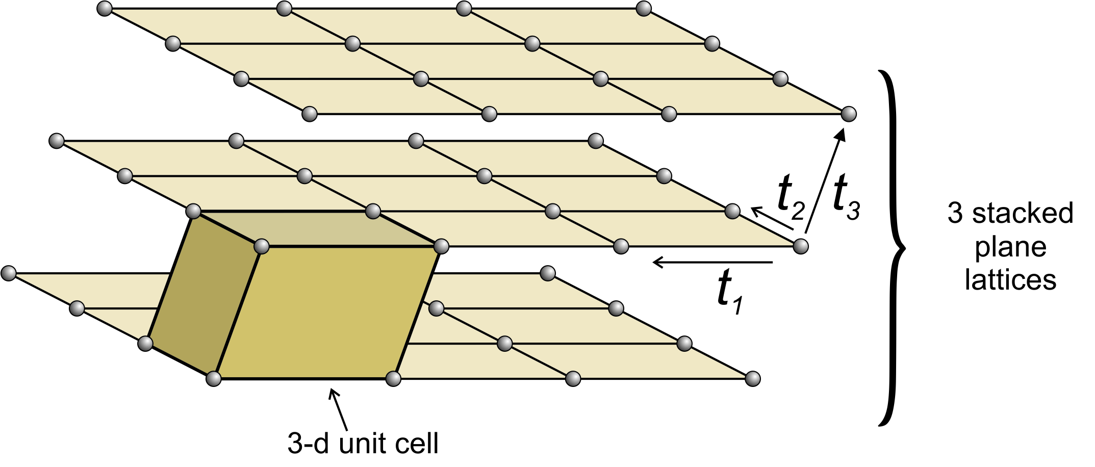
Figure 11.35 shows an example of losing symmetry when nets are stacked with an offset. In this figure, we started with an orthonet. The third translation (t3) is neither perpendicular to, nor of the same magnitude as, either of the other two. Each plane lattice is offset slightly to the right compared with the one below it. The result is a unit cell that has rectangular faces on four sides and parallelograms on two. It is called a monoclinic unit cell (because one angle at each corner is not 90o. An individual orthonet contains mirror planes and 2-fold axes perpendicular to the net. But because, in this example, the third translation was not perpendicular to the first two, those mirrors and rotation axes do not persist in the space lattice, nor in the unit cell. The orthonet has symmetry 2mm; the unit cell has symmetry 2/m. The 2/m axis is perpendicular to the front parallelogram face.
If we consider all possible combinations of plane lattices and a third translation, we come up with seven fundamental unit cell shapes (Figure 11.36). Two of the unit cells, the hexagonal prism and the rhombohedron, are commonly grouped because they both derive from stacking hexanets. If we stack hexanets one above another, we preserve the 6-fold rotation axis and get a hexagonal prism. If the nets are offset, we may instead preserve a 3-fold rotation axis and get a rhombohedron.
You can think of these 3D shapes as the shapes that bricks can have if they fit together without spaces between them. We made a similar analogy to tiles when we were looking at 2D symmetry earlier in this chapter. Just like the tile shapes, more complex brick shapes are possible. But it can be shown that they are all equivalent to one of the seven below.
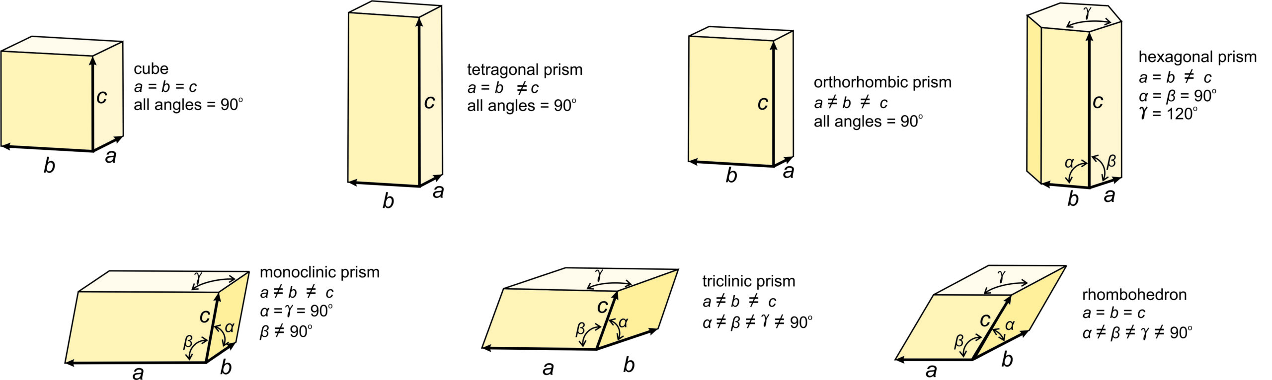
These seven unit cell shapes have unique symmetries: 4/m32/m (cube), 4/m2/m2/m (tetragonal prism), 2/m2/m2/m (orthorhombic prism), 6/m2/m2/m (hexagonal prism), 2/m (monoclinic prism), 1 (triclinic prism), and 32/m (rhombohedron). With one exception, each unit cell corresponds to the one of the seven crystal systems introduced in the previous chapter: cubic, tetragonal, orthorhombic, hexagonal, monoclinic, triclinic, and trigonal. The exception is that some minerals with a hexagonal unit cell crystallize to form trigonal crystals. Common quartz (low quartz) is an example. Its unit cell is hexagonal, but quartz crystals have symmetry 32. (See Box 11-4.) An additional complication sometimes arises because the atomic arrangements in crystals with a rhombohedral unit cell may be described using a much larger hexagonal unit cell.
The symmetry of each unit cell seen in Figure 11.36 is the same as the symmetry of the general form in each system. A third law of crystallography is that:
blank ■The symmetries of the unit cells are the same as the point groups of greatest symmetry in each of the crystal systems.
All minerals that belong to the cubic system have cubic unit cells with symmetry 4/m32/m. Their crystals, however may have less symmetry. Similarly, all minerals that belong to the tetragonal system have tetragonal unit cells. Tetragonal crystals may have 4/m2/m2/m symmetry but may have less. This same kind of thinking applies to crystals in the other 5 systems, too.
We describe the shapes of unit cells with unit cell parameters that include a, b, and c, the length of unit cell edges, and α, β, and γ, the angles between cell edges. By convention, the angle between the a and b edges is γ (c in the Greek alphabet), the angle between a and c is β (b in the Greek alphabet), and the angle between b and c is α (a in the Greek alphabet). As seen in Figure 11.36, in cubic unit cells, a, b, and c are equal, and all angles are 90o. In tetragonal unit cells, a and b are equal and all angles are 90o. In orthorhombic unit cells, the three cell edges have different lengths, but all angles are 90o. In hexagonal unit cells, a and b have equal lengths, and the angle between a and b (γ) is 120o. In monoclinic unit cells, a, b and c are all different. α and γ are 90o, but β can have any value. (This is the general convention, but sometimes the non-90o angle is chosen as one of the other angles instead of β.) In triclinic unit cells, all cell edges are different lengths and all angles are different and not 90o. And in rhomb-shaped unit cells, the cell edges are all the same length, and the angles at the corners are the same for all faces, but are not 90o.
The seven distinct unit cell shapes shown above in Figure 11.35 are all that are possible. The seven are primitive – they contain one lattice point in total. But stacking plane lattices can lead to other, nonprimitive, unit cells that have one of the seven shapes we have seen. Figure 11.36 shows three examples.
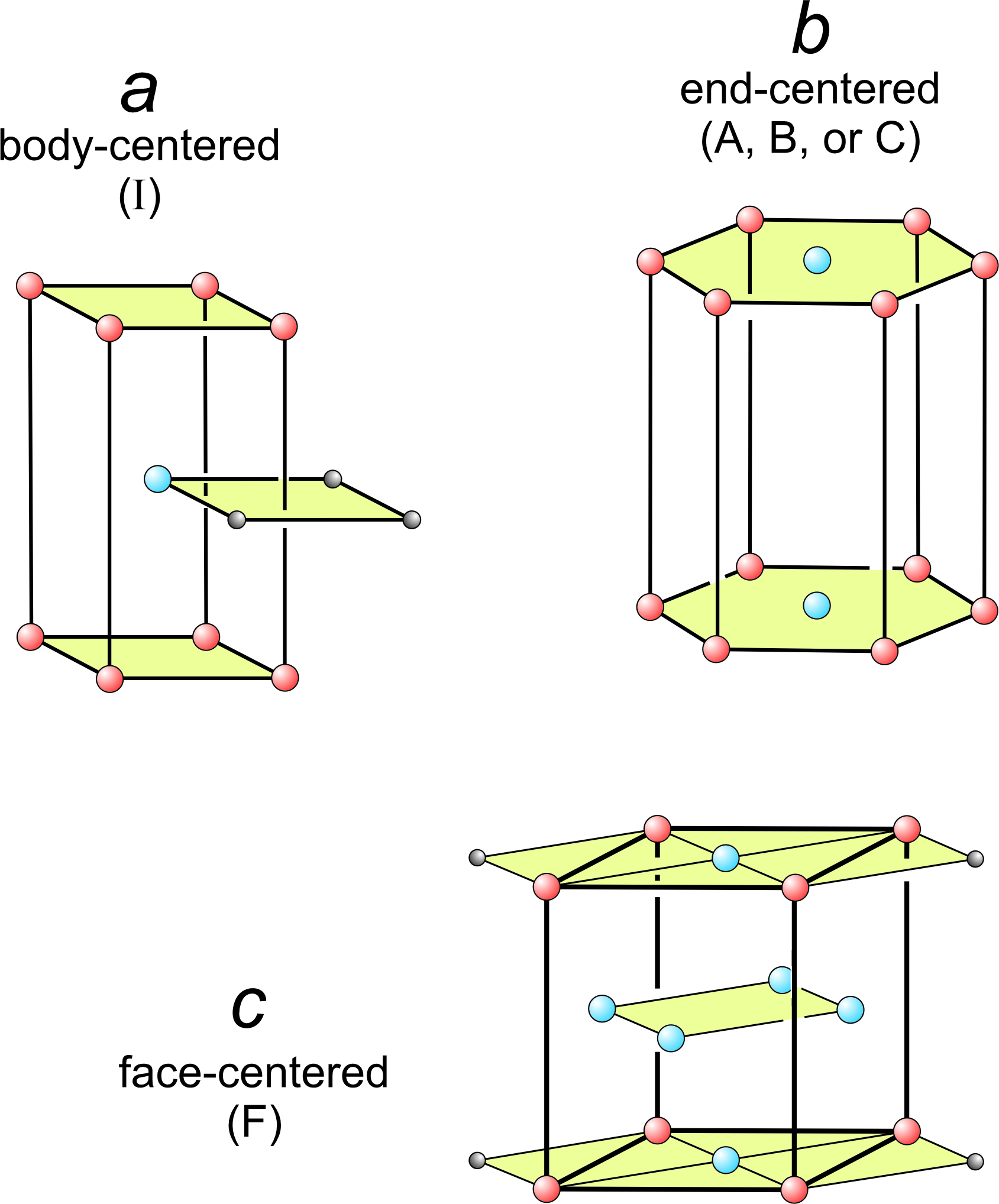
In Figure 11.37a, square nets have been stacked so that every other net is offset. One square from each of three layers is shown. The offset layer puts an extra lattice point (blue) in the center of a tetragonal prism. This is an example of a body-centered unit cell, symbolized by the letter I.
In Figure 11.37b, we put a hexanet directly above another. The result is a hexagonal prism with extra lattice points (blue) in the centers of its top and bottom. This is an example of an end-centered unit cell, symbolized by the letters A, B, or C, depending on which pair of faces contain the extra lattice points.
In Figure 11.37c, diamond nets are stacked with the middle layer offset. This produced an orthorhombic prism that contains extra lattice points at the centers of every face. This is an example of a face-centered unit cell, symbolized by the letter F.
11.4.1 Bravais Lattices

When all possibilities have been examined, we can show that only 14 distinctly different space lattices exist. We call them the 14 Bravais lattices, named after Auguste Bravais, a French scientist who was the first to show that there were only 14 possibilities. The 14 Bravais lattices correspond to 14 different unit cells that may have any of seven different symmetries.
Figure 11.38 lists the 14 Bravais lattices and shows a unit cell for each. In this figure, red lattice points are at the corners of unit cells and blue spheres are the extra points due to centering. Symbols such as 1P, 2P, 2C, 222P, etc., beneath each figure describe their symmetries and whether they are primitive (P) or centered (I, F, A, B, C). These are the standard labels we use for each of the 14 lattices.
Seven of the possible unit cells are primitive (P), one in each system (shown in Figure 11.35). In these unit cells, eight cells share each of the eight lattice points at the corners, so the total number of lattice points per cell is one.
The other eight Bravais lattices involve nonprimitive unit cells containing two, three, or four lattice points. Body-centered unit cells (I), for example, contain one extra lattice point at their center (Figure 11.37a). End-centered unit cells (C) contain extra lattice points in two opposite faces (Figure 11.37b). But the extra points are only half in the cell, so the total number of lattice points is 2. Face-centered unit cells (F) have lattice points in the centers of six faces (Figure 11.37c). Each of the six points is half in the unit cell and half in an adjacent cell. The total number of lattice points is therefore 1 (at the corners) + 3 (in the faces) = 4.
As pointed out in the discussion of two-dimensional lattices, we sometimes make arbitrary decisions when choosing unit cells. The 14 Bravais lattices, in fact, do not represent the only 14 that we could list. For example, in the monoclinic system, the end-centered (2F) unit cell is equivalent to a body-centered one (2I) with different dimensions. Most crystallographers consider only the end-centered cell because that is the way it has been done since the time of Bravais. The important thing to realize is that no matter what unit cells and lattices we consider, only 14 are distinct. Furthermore, the 14 in Figure 11.38 are the simplest and the ones used by most crystallographers.
For a good discussion of Bravais Lattices, watch this video:
blank▶️ Video 11-1: Bravais Lattices (6 minutes)
11.4.2 Unit Cell Symmetry and Crystal Symmetry
Consider fluorite (CaF2), spinel (MgAl2O4), the garnet almandine (Fe3Al2Si3O12), and the rare mineral tetrahedrite (Cu12As4S13). Tetrahedrite has a primitive cubic unit cell; fluorite and spinel have face-centered cubic unit cells; almandine has a body-centered cubic unit cell. In fluorite, Ca2+ is found at the corners of the unit cell and at the center of each face, while F–occupies sites completely within the unit cell (see Figure 11.6). Spinel, almandine, and tetrahedrite have more complex structures, in large part because they contain more than one cation.
Many unit cells together make up a crystal. The crystal may or may not have the same symmetry as a single unit cell. In fluorite, spinel, and almandine crystals, unit cells stack together so that all symmetry elements (rotation axes and mirror planes) are preserved. However, fluorite crystals are typically cubes, spinel crystals are typically octahedra, and almandine crystals are typically dodecahedra. Figure 11.38 shows how cubes can combine to make these shapes. Figure 11.38e shows an example of a crystal, made with a cubic unit cell, that contains two forms (two differently shaped kinds of faces).
Figures 11.40 through 11.43 show mineral examples. We also saw a beautiful dodecahedral garnet crystal in Figure 10.48 (Chapter 10) and well formed fluorite crystals in Figures 4.3 and 4.37 (Chapter 4). The cube, octahedron, and dodecahedron are all special forms that have the same symmetry as the unit cell, 4/m32/m. Tetrahedrite crystals (Figures 11.39d and 11.43), in contrast with the other three, do not have the same symmetry as their unit cell. Although made of cubic unit cells, the crystals lack 4-fold rotation axes. Instead, when euhedral, tetrahedrite crystals typically form pyramids that have symmetry 43m. See the drawing in Figure 11.39d, below.
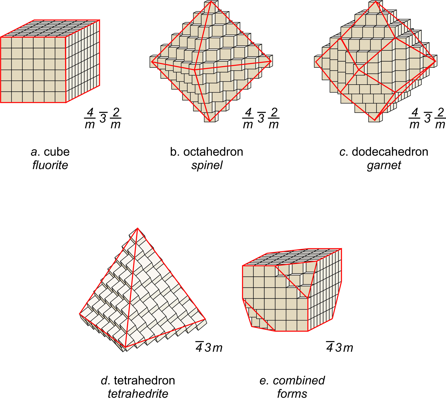
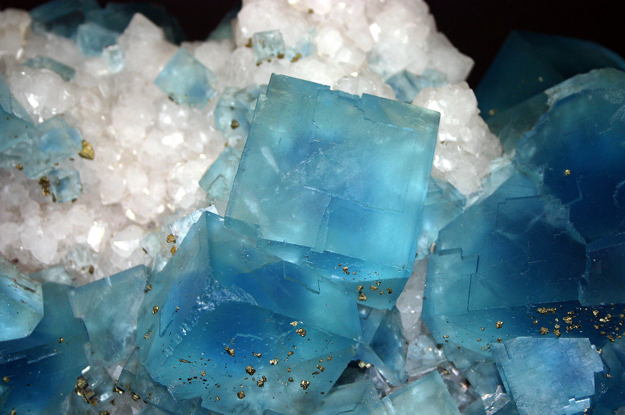
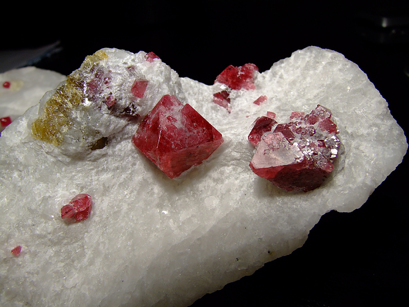
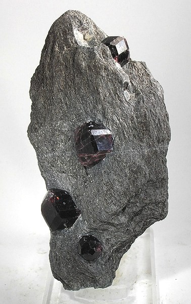
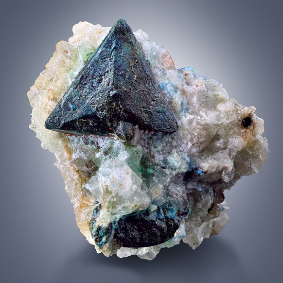
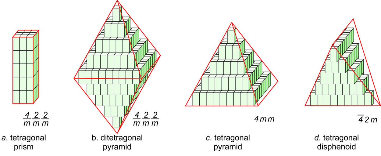
Figure 11.44 shows how tetragonal unit cells can be stacked to produce crystals. The results include a tetragonal prism and a ditetragonal pyramid that have the same symmetry as the unit cell (4/m2/m2/m). But tetragonal unit cells can also create a pyramid (with symmetry 4mm) or a tetragonal disphenoid (with symmetry 42m). Other shapes with other symmetries are possible too. Note that the crystal in Figures 11.44b and d contain a single form (all faces are the same shape); the other two crystals contain two forms.
The preceding discussion points out a fourth important law of crystallography is:
blank■ If a crystal has certain symmetry, the unit cell must have at least as much symmetry.
As a corollary to this law, because crystals consist of unit cells, the symmetry of a crystal can never be more than that of its unit cell. If a crystal has a 4-fold axis of symmetry, it must have a unit cell that includes a 4-fold axis of symmetry. A mineral that forms cubic crystals must have a cubic unit cell. If a crystal has certain symmetry, it is certain that the unit cell and crystal’s atomic structure have at least that much symmetry. They may have more, as in the case of tetrahedrite.
This fourth law is the basis for the crystal systems we introduced in the previous chapter. The symmetry of a crystal requires certain symmetry in the crystal’s unit cell. And we divide the 32 possible symmetries – the 32 point groups – into systems based on that understanding. So we assign crystals to a system based on their symmetry. And crystals in the same crystal system all have the same shaped unit cells, even if the crystals themselves do not look the same. (There is a complication for the trigonal system, discussed later in this chapter.)
If, for example, a crystal has symmetry 4, 4, 4/m, 422, 4mm, 42m, or 4/m2/m2/m, it must have a unit cell that is a tetragonal prism. If a crystal has symmetry 222, mm2, or mmm, it must have a unit cell that is an orthorhombic prism, and so forth. The table below summarizes these relationships. By examining a crystal’s morphology, we can often determine the point group, system, and unit cell shape. Determining whether a unit cell is primitive, face-centered, body-centered, or end-centered, however, is not possible without additional information, which usually comes from X-ray diffraction studies.
| Crystal Systems and Point Groups |
||
| crystal system | unit cell shape | point groups |
| triclinic | triclinic prism | 1, 1 |
| monoclinic | monoclinic prims | 2, m, 2/m |
| orthorhombic | orthorhombic prism | 222, mm2 , mmm |
| tetragonal | tetragonal prism | 4, 4, 4/m, 422, 4mm, 42m, 4/m2/m2/m |
| trigonal | rhombohedron or hexagonal prism | 3, 3, 32, 3m, 3 2/m |
| hexagonal | hexagonal prism | 6, 6, 6/m, 622, 6mm, 62m, 6/m2/m2/m |
| cubic | cube | 23, 2/m3, 432, 43m, 4/m32/m |
It is important to remember that the symmetry of a crystal depends not only on the symmetry of the unit cell, but also on how the unit cells combine to make the crystal. Some minerals, such as halite and other salts, tend to develop euhedral crystals with obvious symmetry, making it easy to infer the symmetry of the unit cell. Others develop crystals with faces that are nearly identical, suggesting the presence of symmetry but leaving some uncertainty. While size and shape of faces can vary because of accidents of crystal growth, the angles between faces vary little from the ideal (Steno’s law). Consequently, crystallographers often rely on angles instead of face shapes to infer the symmetry of the unit cell. Even if a crystal is anhedral and poorly formed, its internal structure is orderly and its unit cells all have the same atomic arrangement.
11.5 Symmetry of Three Dimensional Atomic Arrangements
In the preceding sections, we discussed the shapes and symmetries of crystals. We now turn our attention briefly to space symmetry, the symmetry of three-dimensional atomic structures. What possible symmetry can be present? An atomic arrangement in a crystal consists of groups of atoms (an atomic motif) that repeat an infinite number of times according to one of 14 space lattices. Thus, the overall symmetry depends on both the symmetry of atoms in a motif and the lattice type.
Atomic motif symmetry may involve rotation axes, rotoinversion axes, mirror planes or inversion centers. So motifs may have symmetries equivalent to any of the 32 point groups. Consider an orthorhombic mineral, for example. Its atomic motif may have symmetry mmm, 2/m2/m2/m, or mm2. Its lattice may be 222P, 222C, 222I, or 222F. That gives 12 possible combinations. If we do this calculation for all crystal systems, we come up with 61 possible symmetries for 3D atomic arrangements. We call these space symmetries because they describe the symmetries of atoms in 3D space (as opposed to point symmetries that describe the symmetry of a crystal or motif). Each of the 61 contains a unique combination of symmetry elements. There are, however, many more than 61 because in 3D, we have additional kinds of symmetry operators that we have not considered in detail previously.
11.5.1 Space Group Operators
In 3D, we assign an atomic arrangement to a space group, based on the arrangement’s space symmetry. Each space group is characterized by a combination of one of the 14 Bravais lattices with an atomic motif that has a particular symmetry. We call the different kinds of possible symmetry operators, collectively, space group operators. These operators include the same proper rotation axes, rotoinversion axes, and mirror planes that describe point group (crystal) symmetry. They also include glide planes and screw axes. The addition of glide planes and screw axes is because space symmetry involves translation; point symmetry (crystal symmetry) does not.
11.5.1.1 Glide Planes
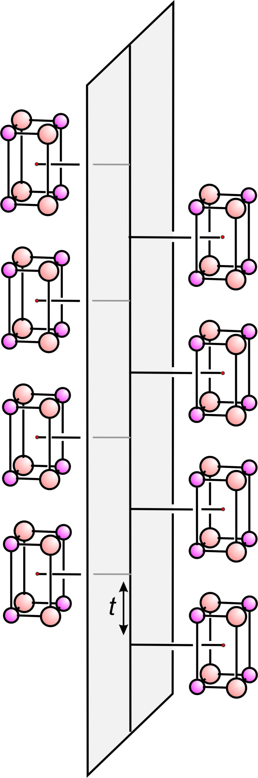
Glide planes differ from normal mirror planes because they involve translation combined with reflection. Earlier in this chapter, we saw examples of glide planes in two dimensions. Figure 11.45 shows a glide plane in three dimensions. A motif of 8 atoms repeats by vertical translation (t) and reflection. This figure involves a simple motif with lots of space around it. The arrangements of atoms in most minerals are generally more complicated and difficult to draw in 3D in a way that shows their symmetries clearly. In part, this is because a glide plane affects all atoms in a structure, not just the ones adjacent to the plane as seen in this figure.
Space group operators combine in many ways. For example, Figure 11.45 contains a vertical glide plane. It also contains horizontal mirror planes. They are proper mirror planes (no glide), perpendicular to the glide, that run through the centers of the 8-atom motifs. Also, although a lot more difficult to see, this atomic arrangement contains horizontal 2-fold rotation axes within the glide plane. The combination of a glide plane and a perpendicular mirror plane requires that the 2-fold axes be present.
Atomic arrangements may contain any of six symmetry elements involving reflection, singly or in combination (table below). These include proper mirror planes and 5 different kinds of glide planes. The glide planes may have any of the orientations that mirror planes can have. The direction of glide may be parallel to the a-, b-, or c-axis, parallel to a face diagonal, or parallel to a body diagonal. In all there are a dozen possibilities.
The direction of gliding distinguishes different types of glide planes and allows us to classify them as axial glides (a-, b-, or c-glides), diagonal glides (n-glides), or diamond glides (d-glides). Some tabulations list an additional kind of glide, an e-glide. E-glides are equivalent to combinations of other glides planes. The table below summarizes the standard possibilities. For most glide planes, the magnitude of the translation (t) is half the unit cell dimension in the direction of translation.
| Space Symmetry Operators Involving Reflection | |||
| operator | type of operation | orientation of translation | translation* |
| m-glide plane a-glide plane b-glide plane c-glide plane n-glide plane d-glide plane |
proper mirror axial glide axial glide axial glide diagonal glide diamond glide |
none parallel to a parallel to b parallel to c par. to a face diagonal par. to main diagonal |
none 1/2 a 1/2 b 1/2 c 1/2 t 1/4 t |
| *a, b, c, and t are the unit cell dimension in the direction of translation |
|||
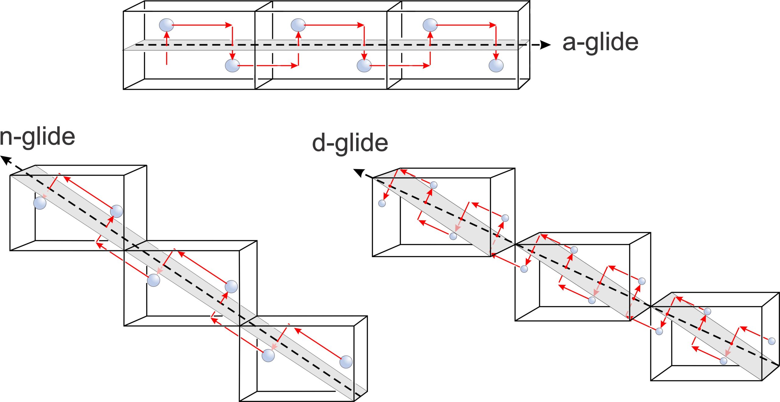
Figure 11.46 compares examples of an a-glide, an n-glide, and a d-glide. Each drawing shows three unit cells. In these examples, the motif contains a single atom. Although these examples contain only one repeating atom, if a glide plane is present in a crystal, all atoms must repeat according to the glide.
The a-glide is relatively easy to see. The atom moves parallel to the cell edge before being reflected across the horizontal glide plane. For the n-glide, the atom reflects the same way, but the glide plane is sloping in each cell. It is parallel to face diagonals of unit cells that share edges. The d-glide is a diagonal glide. The unit cells share corners, and the direction of glide follows the main diagonal of each unit cell from a corner to the diagonally opposite corner. For the a- and n-glides, the translation distance is 1/2 the cell dimension in the direction of the glide. For the d-glide, the translation 1/4 the main cell diagonal length. With these translations, all unit cells are identical. N-glides and d-glides require a centered lattice, and are only possible for tetragonal and cubic minerals.
For further discussion of glide planes, check out the video that is linked here:
blank▶️ Video 11-2: Glide planes (7 minutes)
11.5.5.2 Screw Axes
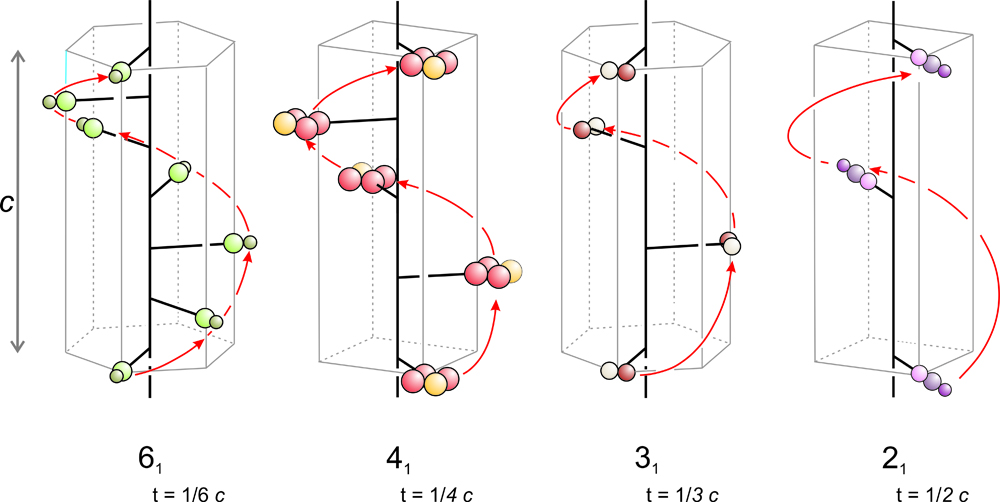
Screw axes result from the simultaneous application of translation and rotation. We combine 2-, 3-, 4-, or 6-fold rotation operators with translation to produce these symmetry operators. Many combinations are possible, and Figure 11.47 shows only a few examples.
A screw axis has the appearance of a spiral staircase. We rotate a motif, translate it, and get an additional motif. As with proper rotation axes (rotation axes not involving translation), each n-fold screw operation involves rotation of 360o/n. After n repeats, the screw has come full circle. The translation associated with a screw axis must be a rational fraction of the unit cell dimension or the result will be an infinite number of atoms, all in different places in different unit cells.
We label screw axes using conventional symbols. In Figure 11.47, they are 61, 41, 31, and 21. In the labels, the large 6, 4, 3, or 2 signifies 6-fold, 4-fold, 3-fold, or 2-fold rotation. The subscript tells the translation distance. A 61 screw axis, for example, involves translation that is 1/6 of the unit cell dimension in the direction of the screw axis. 41, 31, and 21 axes involve translations that are 1/4, 1/3, and 1/2 the unit cell dimension. Similarly, 62, 63, 64, and 65 screw axes (not shown) would involve translations of 2/6, 3/6, 4/6, and 5/6 of the cell dimension.
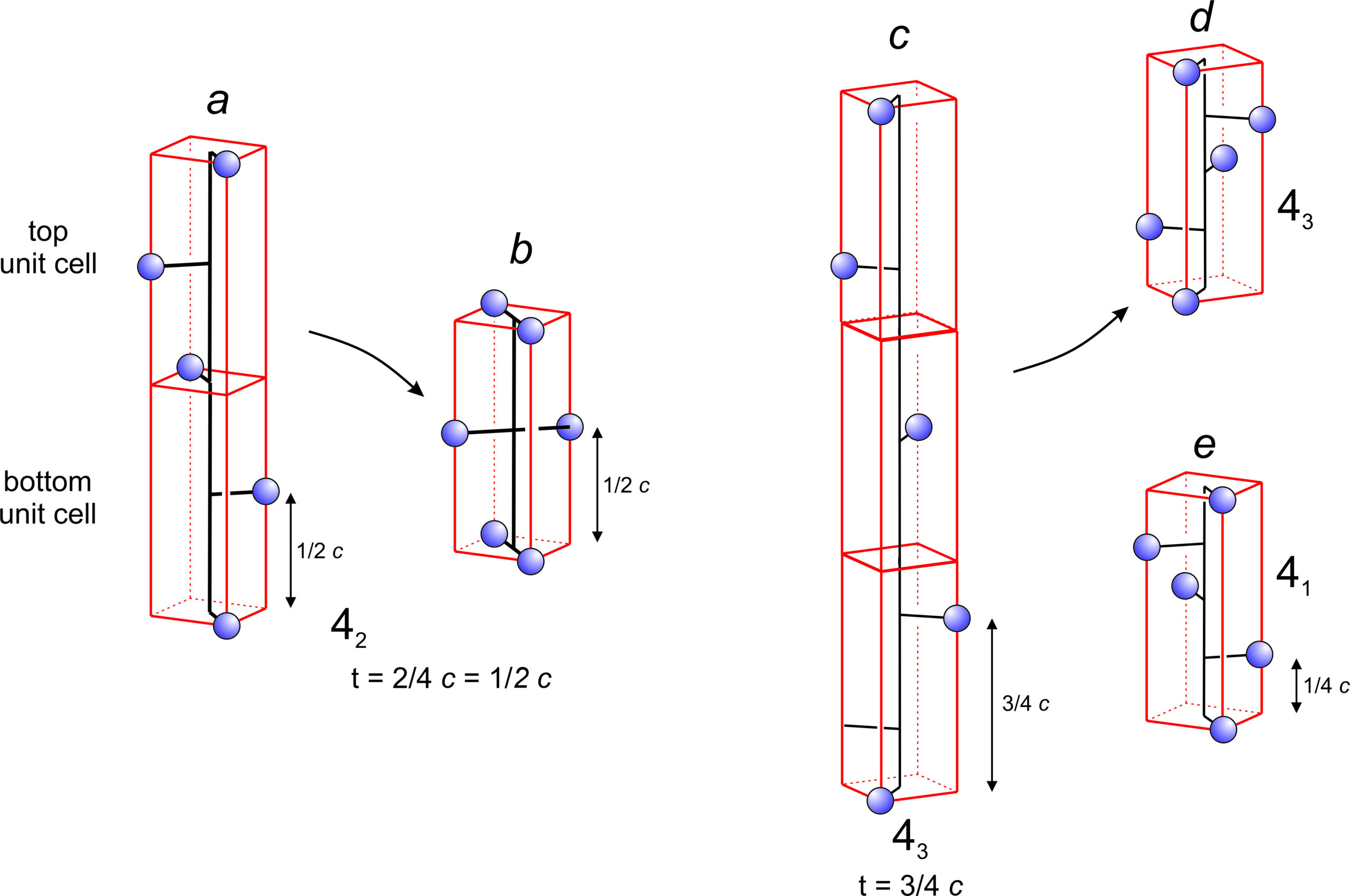
Figure 11.48a shows application of a 42 operator to a single atom. The translation distance is 1/2 the unit cell height (1/2 c), and we must go through four 90o rotations and two unit cells to get another atom that is directly above the starting atom. All unit cells must be identical, but the 42 operation gives a bottom and top unit cell with atoms in different places. The only way this operator can be made consistent is to add the extra atoms shown in Figure 11.48b. In other words, the presence of a 42 axis requires the presence of a 2-fold axis of symmetry.
Figure 11.48c shows a 43 axis and 11.48e shows a 41 axis. After four applications of either operator the total rotation is 360°, bringing the fourth point directly above the first. For the 41 axis, after four applications the total translation is equivalent to one unit cell length. But for the 43 axis it is three unit cell lengths because the translation is 3/4 of the unit cell. All unit cells must be identical, and the only way the 43 operator can be made consistent is to add the extra atoms shown in Figure 11.48d. Note that the 43 and 41 axes produce patterns that are mirror images of each other. The two axes are an enantiomorphic pair, sometimes called right-handed and left-handed screw axes.
When all combinations are considered, we get the 21 possible rotation axes (either proper rotation axes or screw axes) listed in the table below. As with proper rotation axes, some screw axes are restricted to one or a few crystal systems. For example, 31 and 32, which are an enantiomorphic pair, only exist in the trigonal system. Similarly, the 6n axes only exist in the hexagonal system.
| Space Symmetry Operators Involving Rotation | |||
| operator | type of operation | rotation angle | translation* |
| 1 rotation axis 1 rotoinversion axis 2 rotation axis 21 screw axis 2 rotoinversion axis 3 rotation axis 31 screw axis 32 screw axis 3 rotoinversion axis 4 rotation axis 41 screw axis 42 screw axis 43 screw axis 4 rotoinversion axis 6 rotation axis 61 screw axis 62 screw axis 63 screw axis 64 screw axis 65 screw axis 6 |
identity inversion center proper 2-fold 2-fold screw mirror proper 3-fold 3-fold screw 3-fold screw 3-fold rotoinversion proper 4-fold 4-fold screw 4-fold screw 4-fold screw 4-fold rotoinversion proper 6-fold 6-fold screw 6-fold screw 6-fold screw 6-fold screw 6-fold screw 6-fold rotoinversion |
360o 360o 180o 180o 180o 120o 120o 120o 120o 90o 90o 90o 90o 90o 60o 60o 60o 60o 60o 60o 60o |
none none none 1/2 t none none 1/3 t 1/3 t none none 1/4 t 2/4 = 1/2 t 3/4 t none none 1/6 t 2/6 = 1/3 t 3/6 = 1/2 t 4/6 = 2/3 t 5/6 t none |
| *t = the unit cell dimension in the direction of translation | |||
For a further discussion of screw axes, check out the video that is linked here:
blank▶️ Video 11-3: Screw axes (7 minutes)
11.6 Space Groups
When we combine the 32 point groups with the 14 Bravais lattices, and consider all the space group operators in the tables above, we get 230 possible space groups (listed in the Table below; follow this link for a pdf version that is much easier to read). The total number is surprisingly small (see Box 11-2 below, for a discussion). The 230 groups represent all possible symmetries crystal structures can have, although many of them are not represented by any known minerals. Deriving and counting the possible space groups symmetries is not trivial, and crystallographers debated the exact number until the 1890s when several independent studies concluded that there could only be 230. They reached this consensus by applying the mathematical principles of group theory. See Box 11-3 for a brief explanation of group theory and symmetry groups.
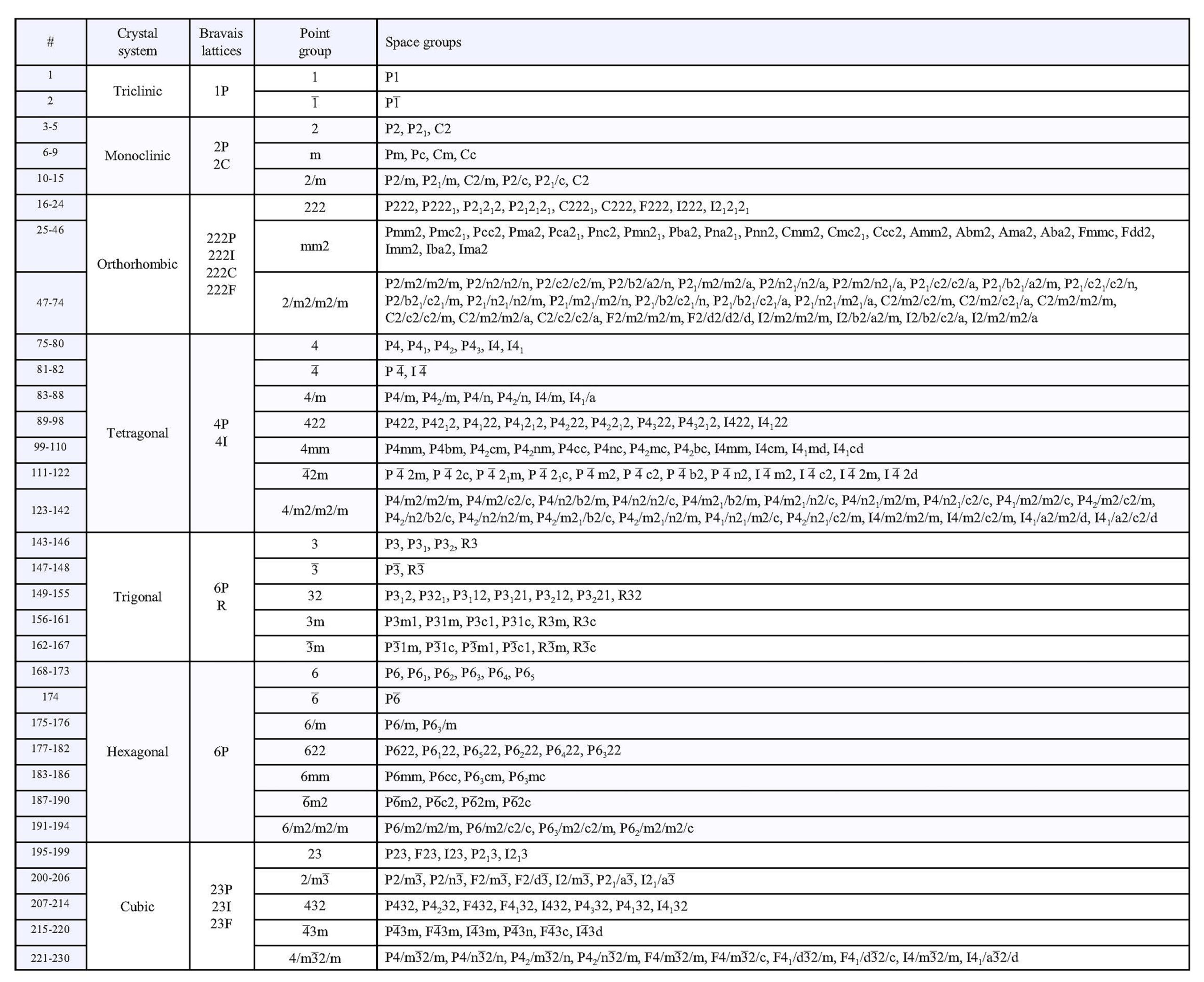
The table above includes complete symmetry symbols for each space group. The space group symbols consist of a letter designating lattice type (P, I, F, R, A, B, or C) followed by symmetry notation similar to conventional Hermann-Mauguin symbols, but with screw axes and glide planes included. Consider, for example rutile. Rutile crystals have symmetry 4/m2/m2/m, but rutile’s space group is P42/m 21/n 2/m. This means that rutile has a primitive (P) tetragonal unit cell, a 42 screw axis perpendicular to a mirror plane, a 21 screw axis perpendicular to an n glide plane, and a proper 2-fold axis perpendicular to a mirror plane. Other minerals have crystals that belong to point group 4/m2/m2/m. Their atomic arrangements, however, may correspond to any of 10 different space groups listed in the table above.
Or consider garnet. Garnet crystals have point group symmetry 4/m32/m. Garnet’s space group is I41/a 3 2/d. This describes a body-centered unit cell (I), a 41 screw axis perpendicular to an a glide plane, a 3-fold rotoinversion axis, and a proper 2-fold axis perpendicular to a d glide plane. There are, however, nine other space groups that can produce crystals with the same symmetry as garnet.
Rather than using an entire space group symbol, crystallographers commonly use abbreviations or symbols to designate the different groups. There are several different ways this is done (see the Wikipedia article on space groups for some comparisons). Thus, they might say that garnet belonged to the space group Ia3d. Abbreviations and shorthand notations, however, can be confusing for those not familiar with the different notation systems, which is why complete symbols are in the table above.
The translations associated with lattices, glide planes, and screw axes are very small, on the order of tenths of a nanometer, equivalent to a few angstroms. Detecting their presence by visual examination of a crystal is impossible, with or without a microscope. A crystal with symmetry 4⁄m2/m2/m could belong to the space group I41/a 2/c 2/d, but there are also 19 other possibilities. We say that the 20 possibilities are isogonal, meaning that when we ignore translation they all have the same symmetry. The table above lists the isogonal space groups for each of the 32 point groups. Without detailed X-ray studies, telling one isogonal space group from another is impossible, and we are left with only the 32 distinct point groups.
For some supplementary information and a different perspective on space groups, check out the video that is linked here:
blank▶️ Video 11-4: Space group operators and space groups (8 minutes)
blank
blank

11.7 Crystal Habit and Crystal Faces
Why do halite and garnet, both cubic minerals, have different crystal habits? It is not fully understood why crystals grow in the ways they do. Cubic unit cells may lead to cube-shaped crystals such as typical halite crystals, octahedral crystals such as spinel, dodecahedral crystals such as garnet, and many other shaped crystals. Why the differences? Crystallographers do not have complete answers, but the most important factor is the location of atoms within a unit cell.
Crystals of a particular mineral tend to have the same forms, or only a limited number of forms, no matter how they grow. Haüy and Bravais noted this and used it to infer that atomic structure controls crystal forms. In 1860, Bravais observed what we now call the Law of Bravais:
blank■ Faces on crystals tend to be parallel to planes having a high density of lattice points.
This means that, for example, crystals with hexagonal lattices and unit cells often have faces related by hexagonal symmetry. Crystals with orthogonal unit cells (those in the cubic, orthorhombic, or tetragonal systems) tend to have faces at 90° to each other.
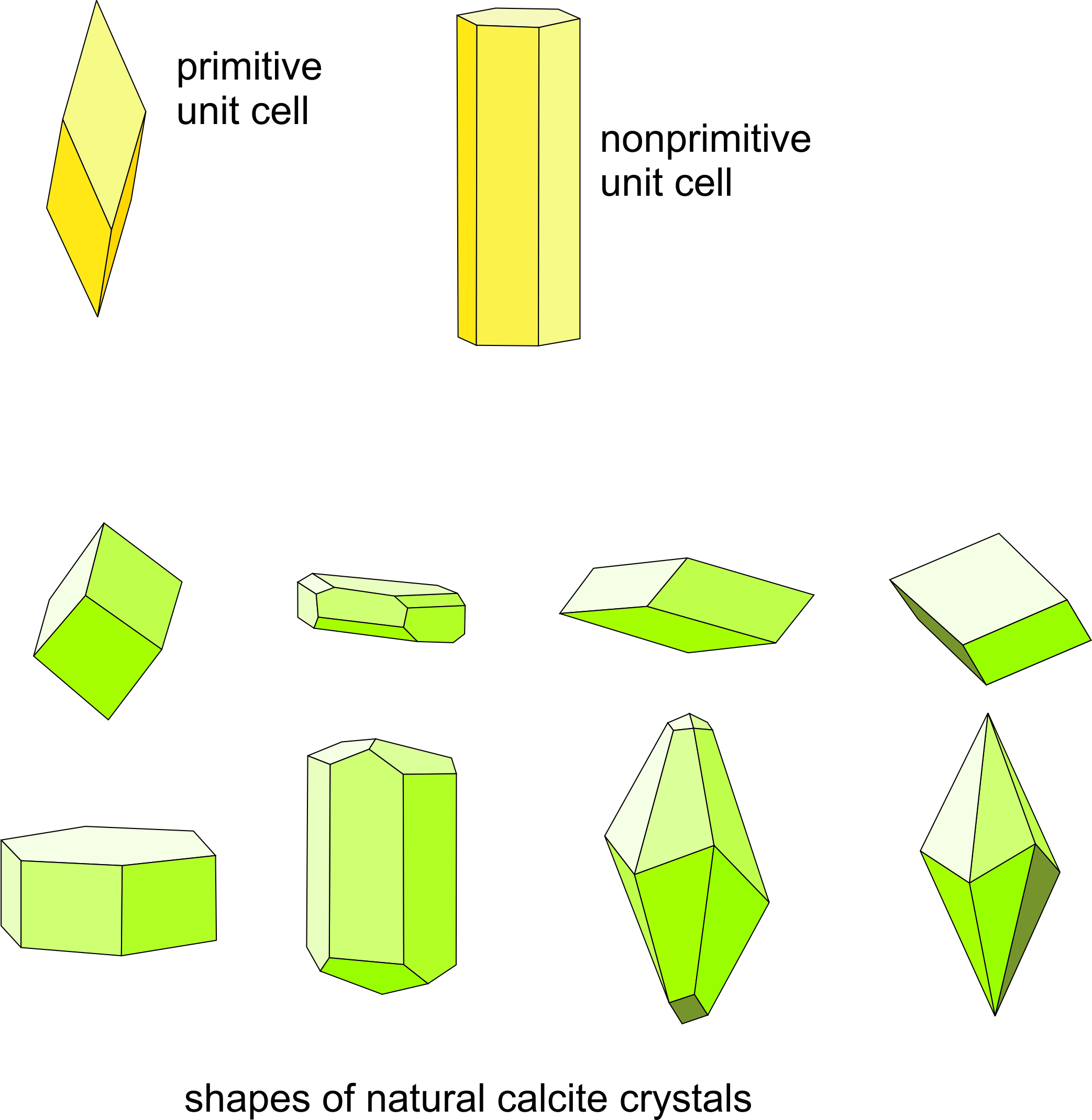
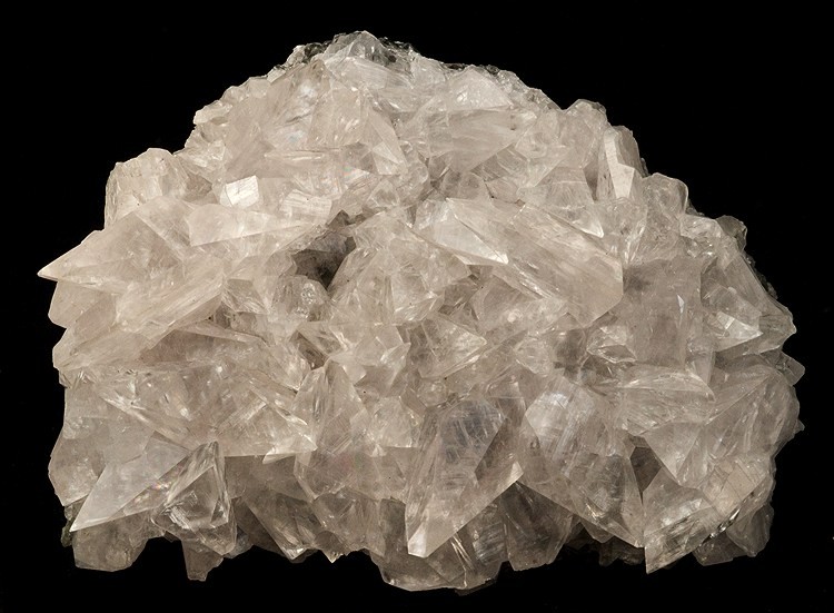
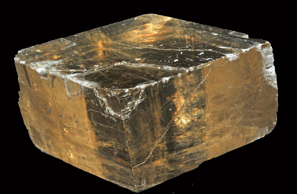
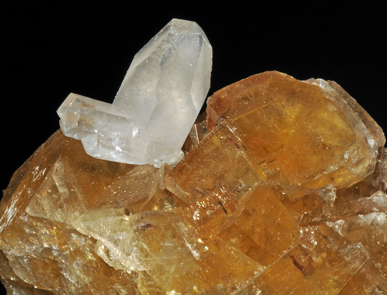
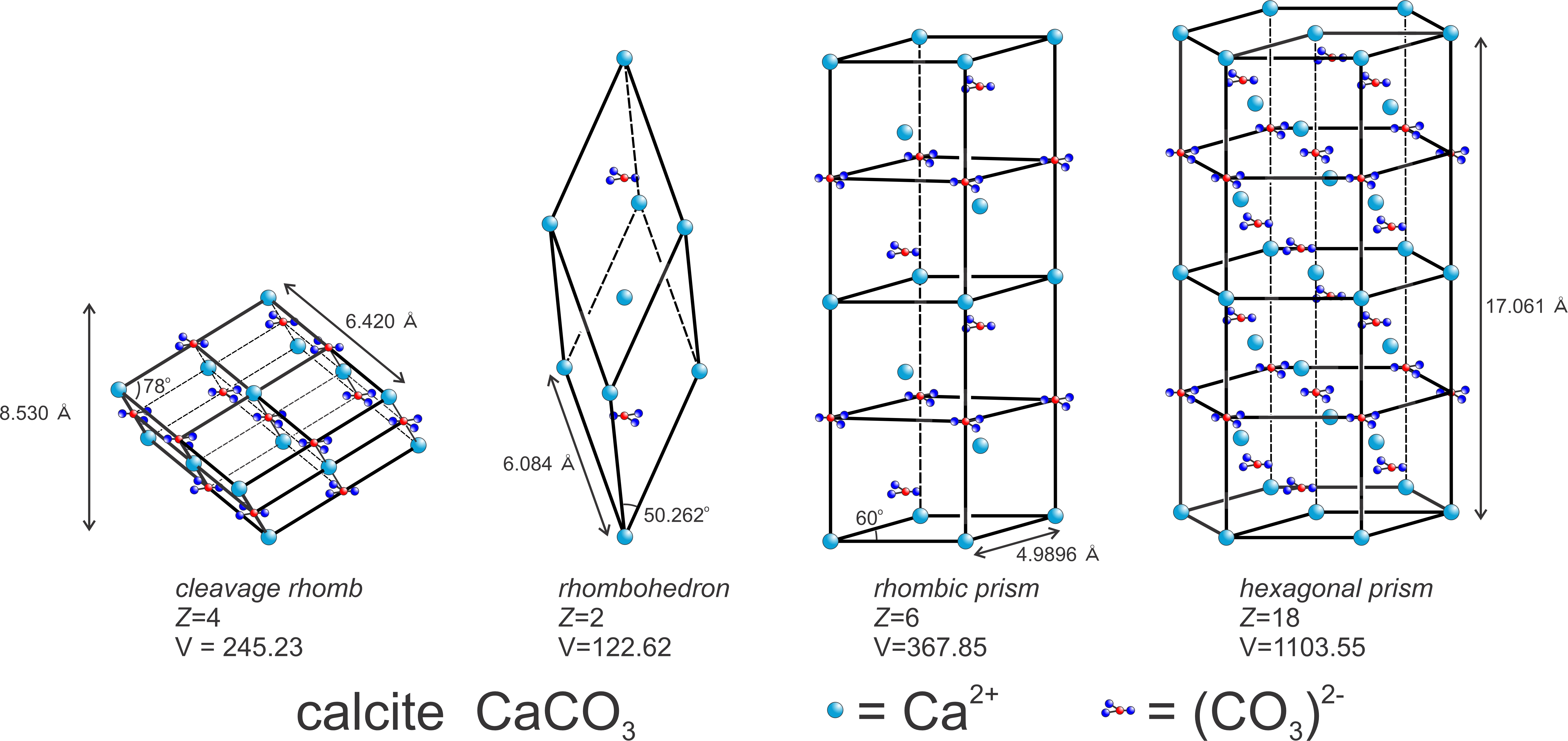
The relationship between lattice/unit cell symmetry and crystal habit can be seen in Figure 11.49. The figure shows two choices for calcite’s unit cell (yellow drawings). The rhombohedron is a doubly primitive unit cell (containing two CaCO3 motifs) and the hexagonal equivalent contains four CaCO3 motifs. The drawings below the unit cells show some common shapes for natural calcite crystals. There is noticeable resemblance between unit cell shapes, which represent the lattice symmetry, and some of the crystal shapes. Thus, Bravais’s Law works well. The photos below in Figures 11.50 – 11.55 show natural calcite crystals that match quite well the drawings in Figure 11.49.
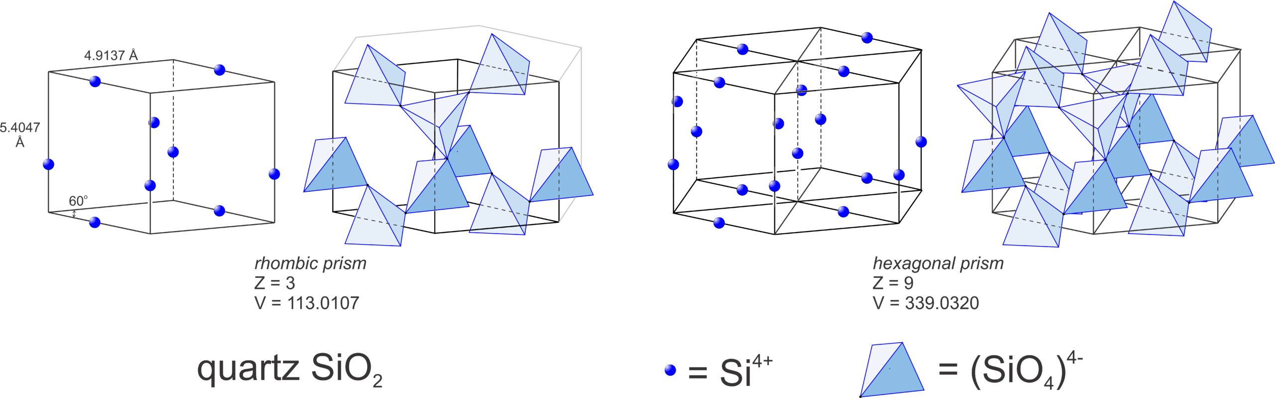
Unfortunately, some minerals, including pyrite (FeS2) and quartz (SiO2), appear to violate Bravais’s Law. Bravais’s observations were based on considerations of the 14 Bravais lattices and their symmetries, but in the early twentieth century, P. Niggli, J. D. H. Donnay, and D. Harker realized that space group symmetries needed to be considered as well. By extending Bravais’s ideas to include glide planes and screw axes, Niggli, Donnay, and Harker explained most of the biggest inconsistencies. They concluded that crystal faces form parallel to planes of highest atom density, a slight modification of the Law of Bravais.
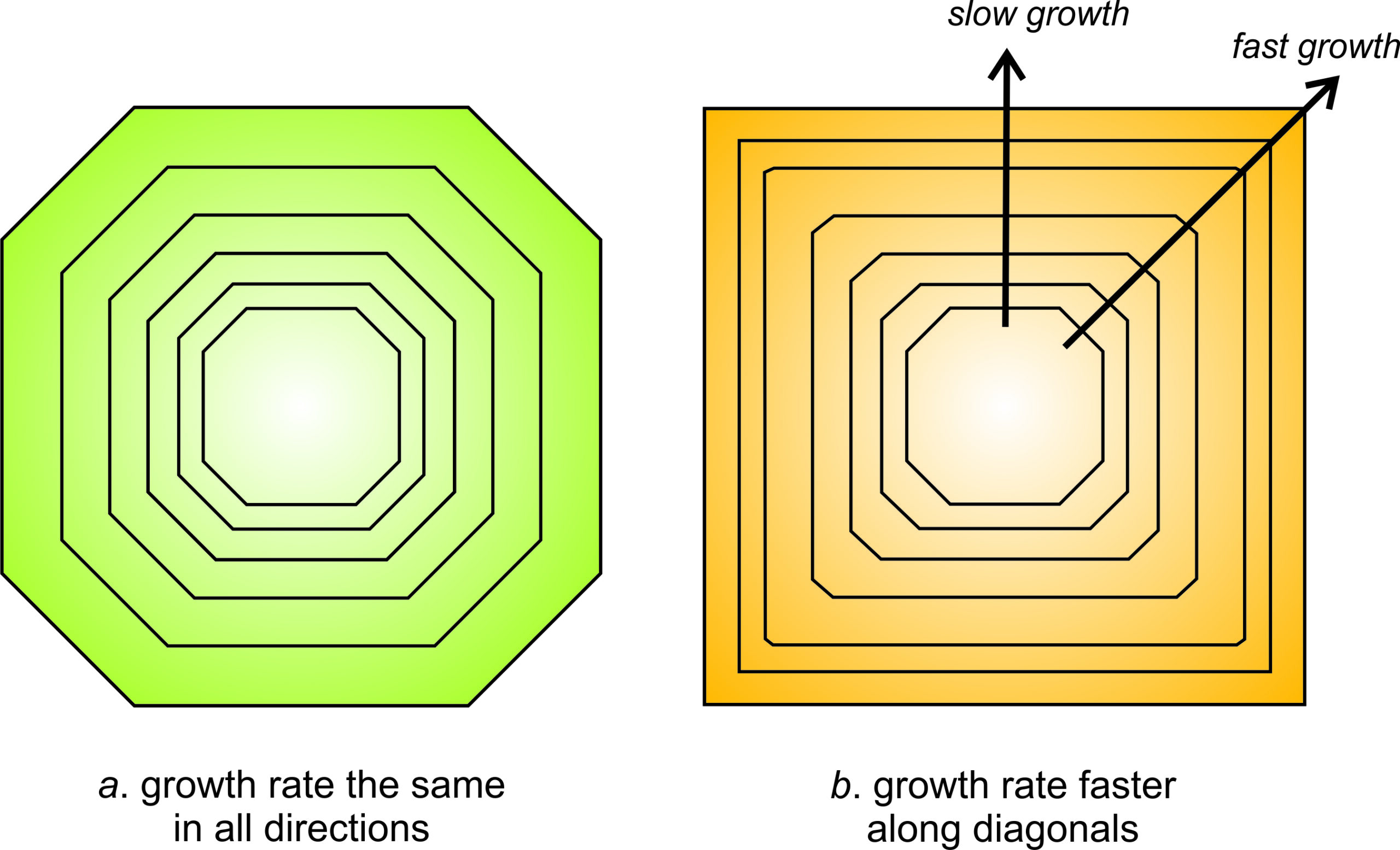
As a crystal grows, different faces grow at different rates. Some may dominate in the early stages of crystallization while others will dominate in the later stages. The relationship, however, is the opposite of what we might expect. Faces that grow fastest are the ones that eventually disappear. Figure 11.56 shows why this occurs. If all faces on a crystal grow at the same rate, the crystal will keep the same shape as it grows (the green crystal in Figure 11.56a). However, this is not true if some faces grow faster than others.
In Figure 11.56b, the diagonal faces (oriented at 45o to horizontal) grew faster than those oriented vertically and horizontally. Eventually, the diagonal faces disappeared; they “grew themselves out.” The final crystal has a different shape, and fewer faces, than when it started growing. We observe this phenomenon in many minerals; small crystals often have more faces than larger ones.
11.8 Quantitative Aspects of Unit Cells, Points, Lines, and Planes
11.8.1 Unit Cell Parameters and Crystallographic Axes
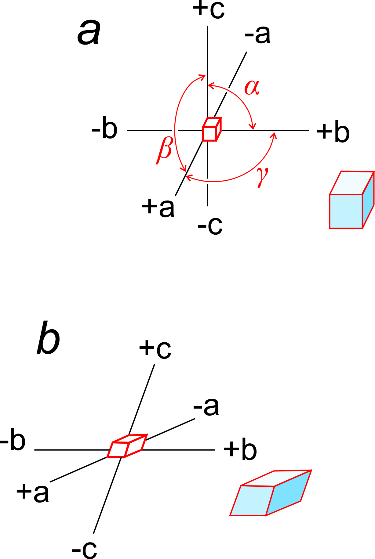
Earlier in this chapter, we introduced the unit cell parameters a, b, c, α, β, and γ. a, b, and c are the lengths of unit cell edges; α, β, and γ are the angles between the edges. α is the angle between b and c, β is the angle between a and c, and γ the angle between a and b (Figure 11.57a).
Unit cell edges define a coordinate system used by crystallographers when they wish to describe the locations of atoms or other features within a cell. Some crystal systems are orthogonal (cubic, tetragonal, orthorhombic) but others are not. Cubic crystals, and others that belong to an orthogonal system, use a standard Cartesian coordinate system. Figure 11.57a shows an example.
Figure 11.57b shows axes that are inclined with respect to each other. In this example, they correspond to a triclinic unit cell. α, β, and γ, the angles between axes, are not equal to 90o and (in contrast with the cube) the edges of the unit cell have different lengths along different axes.
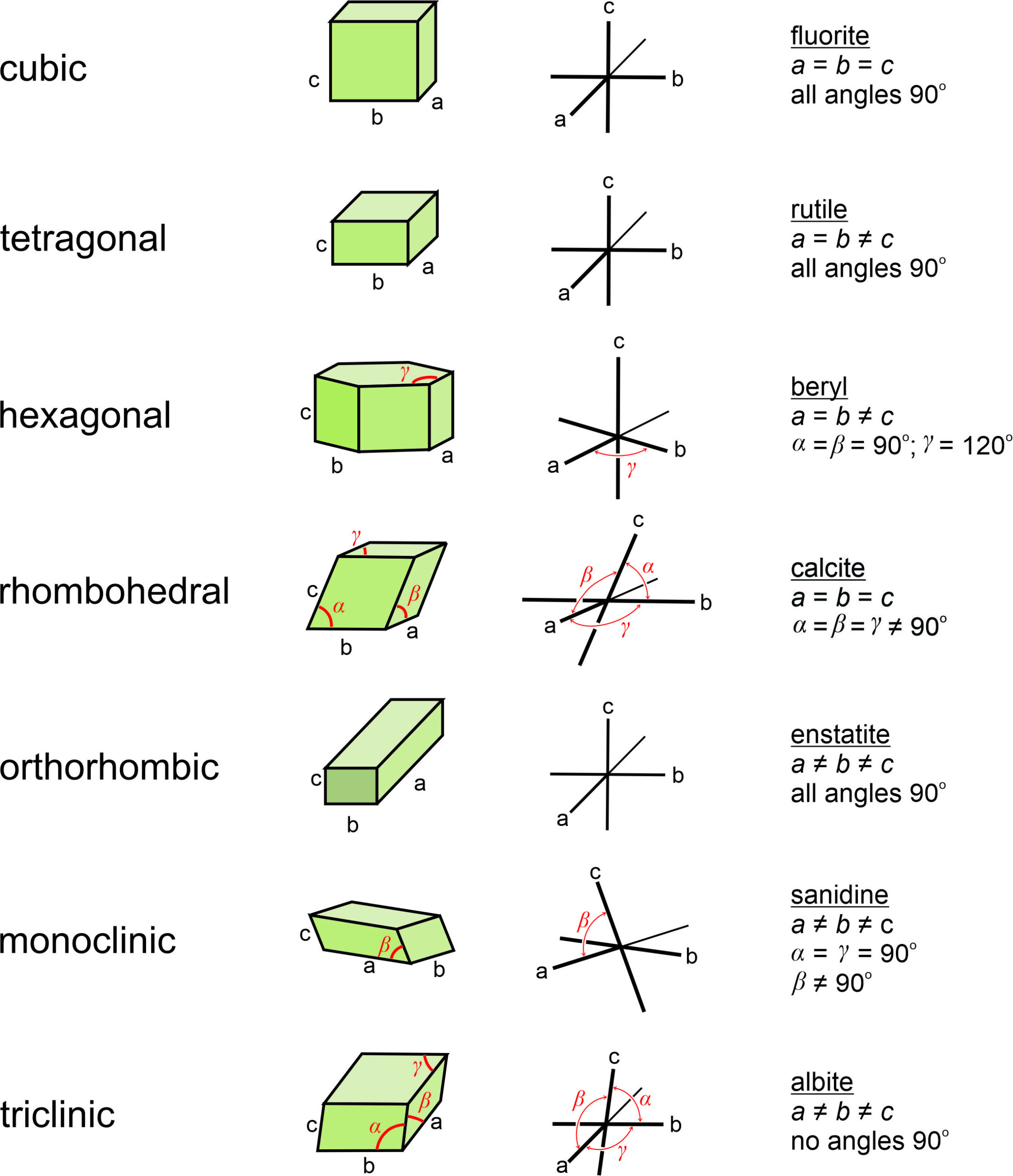
Figure 11.58 shows coordinate axes for each of the seven fundamental unit cell shapes. In the drawings, the non-90o angles are labeled α, β, or γ. For orthogonal unit cells (cubic, tetragonal, orthorhombic), all angles are 90o. For the hexagonal unit cell, β = 120o and the other angles are 90o. For monoclinic unit cells, α and γ are 90o ; β is not.
The right-hand column in Figure 11.58 lists an example mineral for each unit cell, along with the constraints on unit-cell parameters. Unit cells may, however, be chosen in multiple ways. So although we used calcite as an example of a mineral with a rhombohedral unit cell, in much of the literature calcite’s unit cell is described as a prism with rhomb-shaped ends.
Although it makes no practical difference which edges of a unit cell we call a, b, or c, or which angles are α, β, and γ, mineralogists normally follow certain conventions. The restriction on cell parameters in the Table above, and discussed below, are widely accepted guidelines but there are other possibilities. In triclinic minerals, none of the angles are special and a, b, and c are all different lengths. Although the literature contains exceptions, by modern convention edges are chosen so that c < a < b. In monoclinic minerals, such as sanidine, only one angle in the unit cell is not 90°. By convention, the non-90° angle is β, the angle between a and c. For historical reasons, this convention is called the second setting for monoclinic minerals. In orthorhombic crystals, we choose axes so that c > a > b. In tetragonal and hexagonal crystals, the c-axis always corresponds to the 4-fold or 6-fold axis.
In this book we use a, b, and c to designate the three crystallographic axes, but crystallographers sometimes use subscripts to indicate axes, and thus cell edges, that must be identical lengths because of symmetry. Instead of a, b, and c, the three axes of cubic minerals might be designated a1, a2, and a3. The axes of tetragonal crystals can be designated a1, a2, and c.
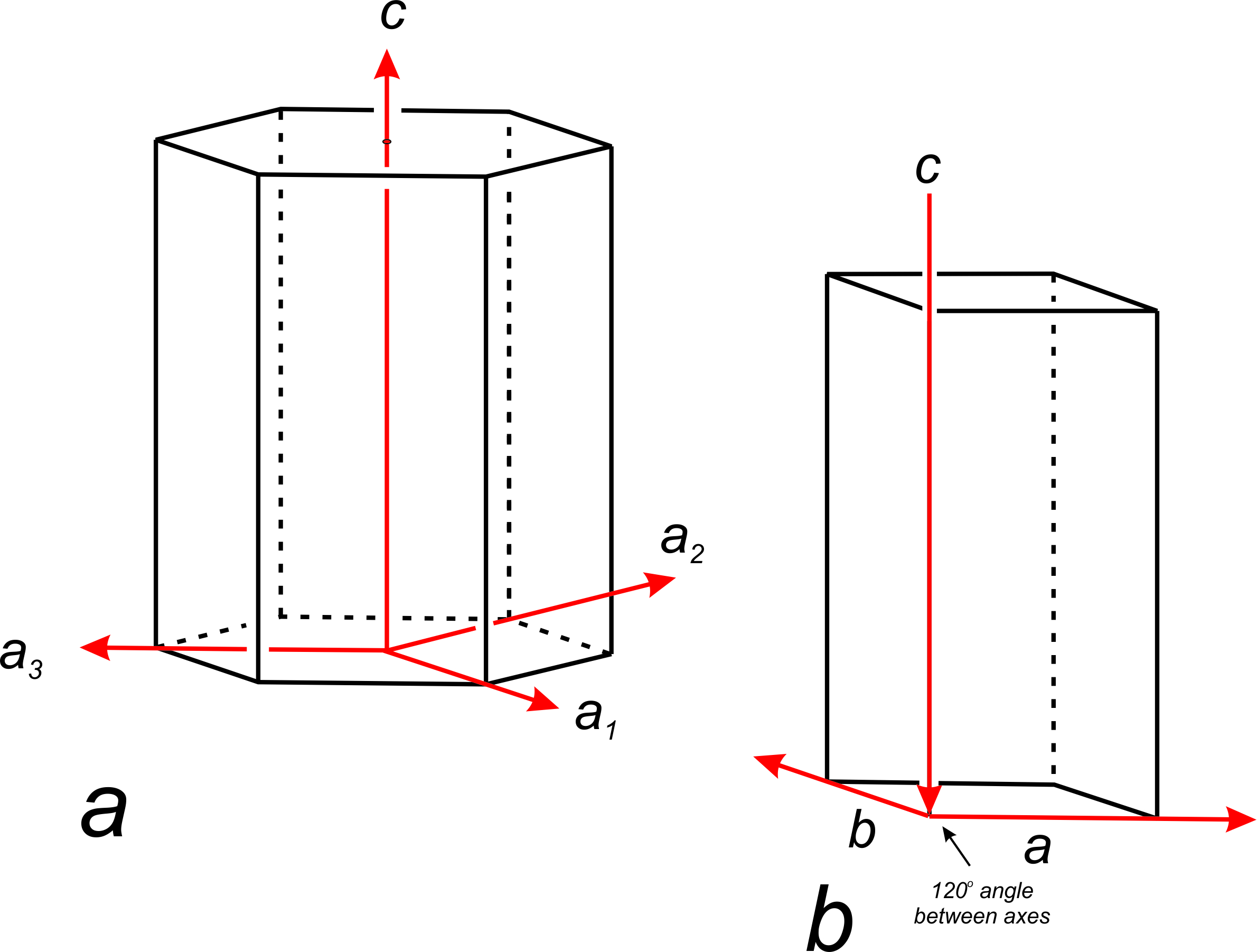
For hexagonal crystals, crystallographers have historically used four axes: a1, a2, a3, and c (Figure 11.59a). The three a-axes, a1, a2, and a3, are parallel to edges of a nonprimitive hexagonal unit cell. Although the third a-axis is redundant for describing symmetry or points in 3D space, it has been included in the past to emphasize that there are three identical a-axes perpendicular to the c-axis. Because only three axes are used in much of the modern literature (Figure 11.59b), we will only briefly mention the fourth axis in the rest of this chapter.
Although mineralogists historically used angstroms (1 Å = 10-10 m) to give cell dimensions, much recent literature uses nanometers (1 nm = 10 Å). Typical mineral unit cells have edges of 2 to 20 Å (0.2 to 2 nm). The angles α, β, and γ are normally given as a decimal number of degrees (for example, 94.62°). These angles between edges vary greatly, although unit cells are often chosen so that angles are close to 90°.
Instead of using angstroms (or nanometers) to give distances, we may also use unit cell dimensions as a scale. For example, we might say that a certain plane intersects the axes at distances of 3a, 2b, and 2c from the origin. It is implicit that 3a refers to a distance equal to three unit cell edge lengths along the a-axis, 2b a distance equal to two unit cell lengths along the b-axis, and 2c a distance equal to two unit cell lengths along the c-axis.
The symmetry of a unit cell always affects the relationships between a, b, and c. So, in the cubic system, a = b = c, but in the tetragonal and hexagonal systems a = b ≠ c. The relationships implied by crystal systems mean that, for systems other than triclinic, we need not give six values to describe unit cell shape. For example, for orthorhombic, hexagonal, tetragonal, and cubic minerals, we do not specify any angles because they are all defined by the crystal system. The table below gives examples of unit cell parameters for minerals from each of the crystal systems; unnecessary information has been omitted. These same example minerals are the ones listed in Figure 11.58.
| Unit Cell Parameters (a, b, c, α, β, and γ), Z (number of formulas per unit cell), and V (unit cell volume) for One Mineral from Each of the Crystal Systems* | ||||||
| fluorite CaF2 |
rutile TiO2 |
beryl Be3Al2Si6O18 |
calcite CaCO3 |
enstatite Mg2Si2O6 |
sanidine KAlSi3O8 |
albite NaAlSi3O8 |
| cubic Z = 4 a = 5.46 V = 162.77 |
tetragonal Z = 2 a = 4.59 c = 2.96 V = 62.36 |
hexagonal Z = 2 a = 9.23 c = 9.19 V = 678.04 |
trigonal Z = 6 a = 4.98 c = 17.06 V = 367.85 |
orthorhombic Z = 4 a = 18.22 b = 8.81 c = 5.21 V = 836.30 |
monoclinic Z = 4 a = 8.56 b = 13.03 c = 7.17 γ = 115.98 V = 799.72 |
triclinic Z = 4 a = 8.14 b = 12.8 c = 7.16 α = 94.33 β = 116.57 γ = 87.65 V = 746.01 |
| *a, b, and c are in angstroms; α, β, and γ are in degrees; and V is in cubic angstroms. The cell parameters for beryl and calcite are for rhombic prisms; sometimes other unit cells are chosen. | ||||||
Consider the triclinic mineral albite, a feldspar with composition NaAlSi3O8. The last column in the table lists albite’s unit cell parameters. Because none of the angles are special and none of the cell edges are equal, we need six parameters to describe the cell shape. In contrast, fluorite (the first column of the table) has a cubic unit cell, so we need to give only one cell dimension, the length of the cell edge. It is implicit that all angles are 90° and all cell edges are the same length.
Physical dimensions do not completely describe a unit cell. We must also specify the nature and number of atoms within the unit cell. To provide some of this information, the table above lists two other things besides dimensions and angles: mineral formulas and Z, the number of formulas in each unit cell. For example, fluorite has the formula CaF2 and Z = 4. This means there are 4 CaF2 molecules (4 Ca and 8 F atoms) in each unit cell. Albite has the formula NaAlSi3O8 and Z = 4. This means that four NaAlSi3O8 formulas are in each unit cell. In other words, each unit cell contains 4 Na atoms, 4 Al atoms, 12 Si atoms, and 32 O atoms.
11.8.2 Points in Unit Cells
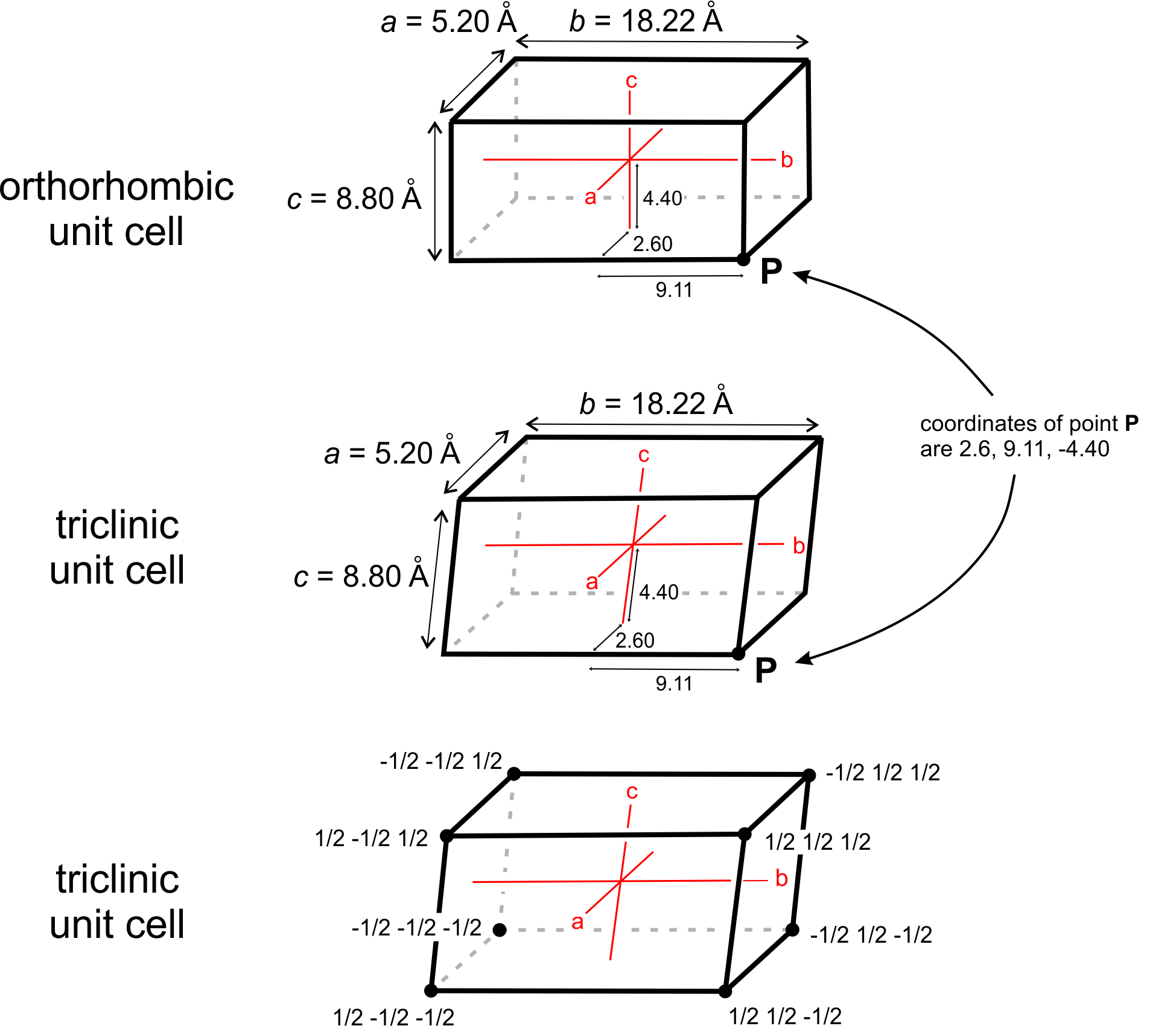
Mineralogists describe the locations of atoms or other points in unit cells by giving their coordinates. As examples, consider the orthorhombic and triclinic crystals shown in Figure 11.60. In the orthorhombic crystal the three axes (shown in red) intersect at 90°, in the triclinic crystal they do not. Assume both crystals have cell dimensions a = 5.20 Å, b = 18.22 Å, and c = 8.80 Å, and the axes’ origins are at the center of the unit cells as shown. The coordinates of point P, at the lower right-hand corner in drawings a and b, are therefore 5.20/2 = 2.60 Å, 18.22/2 = 9.11 Å, and 8.80/2 = -4.40 Å. The negative sign arises because the points are in a negative direction from the origin along the c-axis.
We do not, however, normally report coordinates in angstroms (Å). Instead, we report distances relative to unit cell dimensions. Another way to describe the location of point P in Figure 11.60a and b would be to say it has coordinates 1/2a, 1/2b, -1/2c. Typically, we normalize coordinates to unit cell dimensions by dropping the a, b, and c. The coordinates then become 1/2 , 1/2 , -1/2. The points at the corners must have coordinates ±1/2, ±1/2, ±1/2, if the origin is at the center of the unit cell (Figure 11.60c). Note that the system to which a crystal belongs does not affect coordinate values.
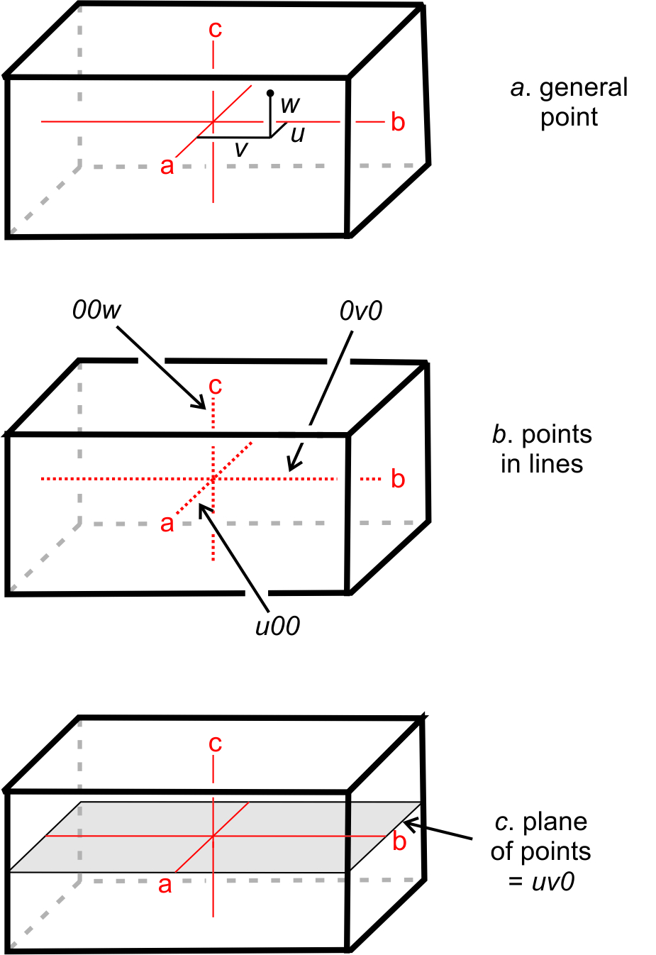
Traditionally, crystallographers have used the variables u, v, and w to represent the coordinates of a point if the coordinates are rational numbers, and x, y, and z if irrational. For simplicity, in this text we will use uvw in all instances (Figure 11.61a). We can say that uvw represents a general point anywhere in the cell.
Suppose two coordinates, for example v and w, are zero. All the points described by the coordinates u00 constitute a set of special points, lying along the a-axis (Figure 11.61b). Similarly, 0v0 and 00w refer to sets of special points on the b- and c-axes, respectively. If only one coordinate equals zero, a point lies in a plane including two axes. We might, for example, talk about special points located at uv0. These are points on a plane that includes the a- and b-axes, as shown in Figure 11.61c. Note that no parentheses or brackets are used when giving coordinates of a point.
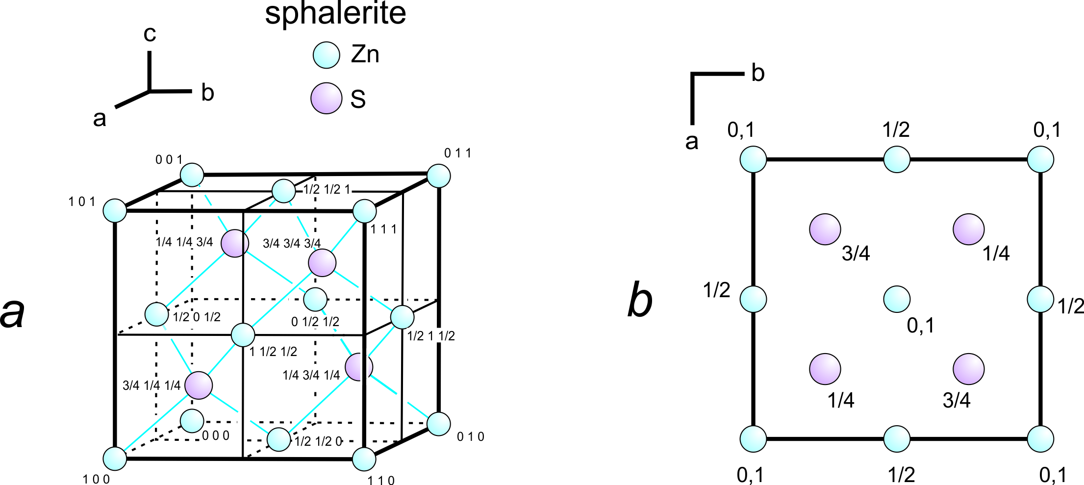
Figure 11.62a shows a unit cell of sphalerite, ZnS, with uvw coordinates for each atom. The axes origin is in the bottom back left corner. Because three-dimensional drawings are sometimes difficult to draw and see, crystallographers often use projections, which contain the same information in a less cluttered manner (Figure 11.62b). In the projection, which is a view down the c-axis, we need not specify u and v values because they can be estimated from the location of the atoms in the drawing. The numbers are w values. Sometimes we omit w values for atoms at unit cell corners; by convention, this means the atoms are found on both the top and bottom of the cell as it appears in projection.
11.8.3 Lines and Directions in Crystals
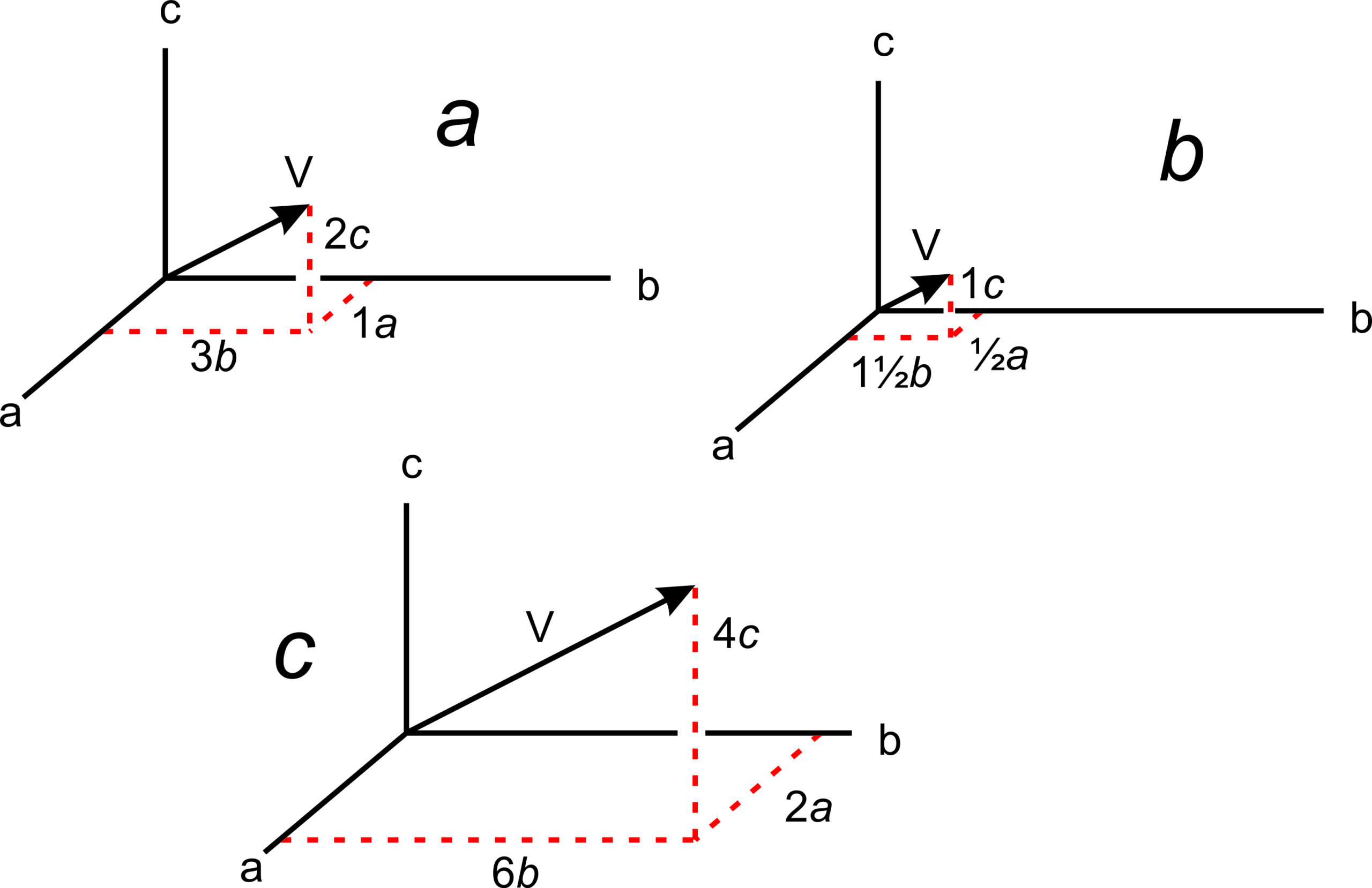
The absolute location of a line in a crystal is not often significant, but directions (vectors) have significance because they describe the orientations of symmetry axes, zones, and other linear features. Crystallographers designate directions with three indices in square brackets, [uvw]. As with point locations, we give numbers describing directions in terms of unit cell dimensions. In Figure 11.63a, direction V has indices [132] – it goes from the origin to a point at 1a, 3b, 2c.
The drawings in 11.63b and 11.63c show other vectors pointing the same direction as [132]. We clear fractions and divide by common denominators when giving the indices of a direction in primitive unit cells. So directions [½ 1½ 1] and [264] would be simplified and described as [132]. Although no commas are included in [132], reading sequentially, as we do for point locations, we articulate it “one-three-two.” By convention, commas separate indices only if they have more than one digit. Note that we do not divide by common denominators when describing directions in centered cells.
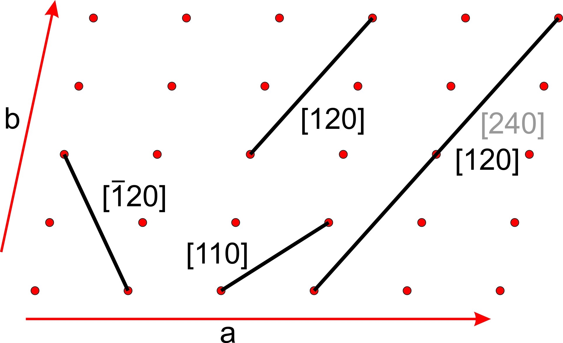
Figure 11.64 shows several lines on a two-a dimensional lattice. Parallel lines have identical indices, and choosing an origin is unimportant. The direction [240] is the same as [120], and when we clear the common denominator [240] becomes [120]. For line [120], the bar over the 1 is equivalent to a negative sign, indicating that the line goes in the negative a-direction. We articulate the indices as “bar-one-two-zero.” Because all directions in Figure 11.64 lie in the a-b plane, they have indices [uv0]. This notation indicates that the first two indices may vary, but the third is 0.
11.8.4 Planes in Crystals
While crystals and crystal faces vary in size and shape, Steno’s law tells us that angles between faces are characteristic for a given mineral. The absolute location and size of the faces are rarely of significance to crystallographers, while the relative orientations of faces are of fundamental importance. We can use face orientations to determine crystal systems and point groups, so having a simple method to describe the orientation of crystal faces is useful.
Figure 11.65a shows three axes with different unit cell lengths; small red dots show unit increments along the axes. The axes are orthogonal, so this arrangement corresponds to the orthorhombic system. Consider a plane parallel to a crystal face. Such a plane may be parallel to one axis (Figure 11.65b), parallel to two axes (Figure 11.64c) or it may intersect all three axes (Figure 11.65d).
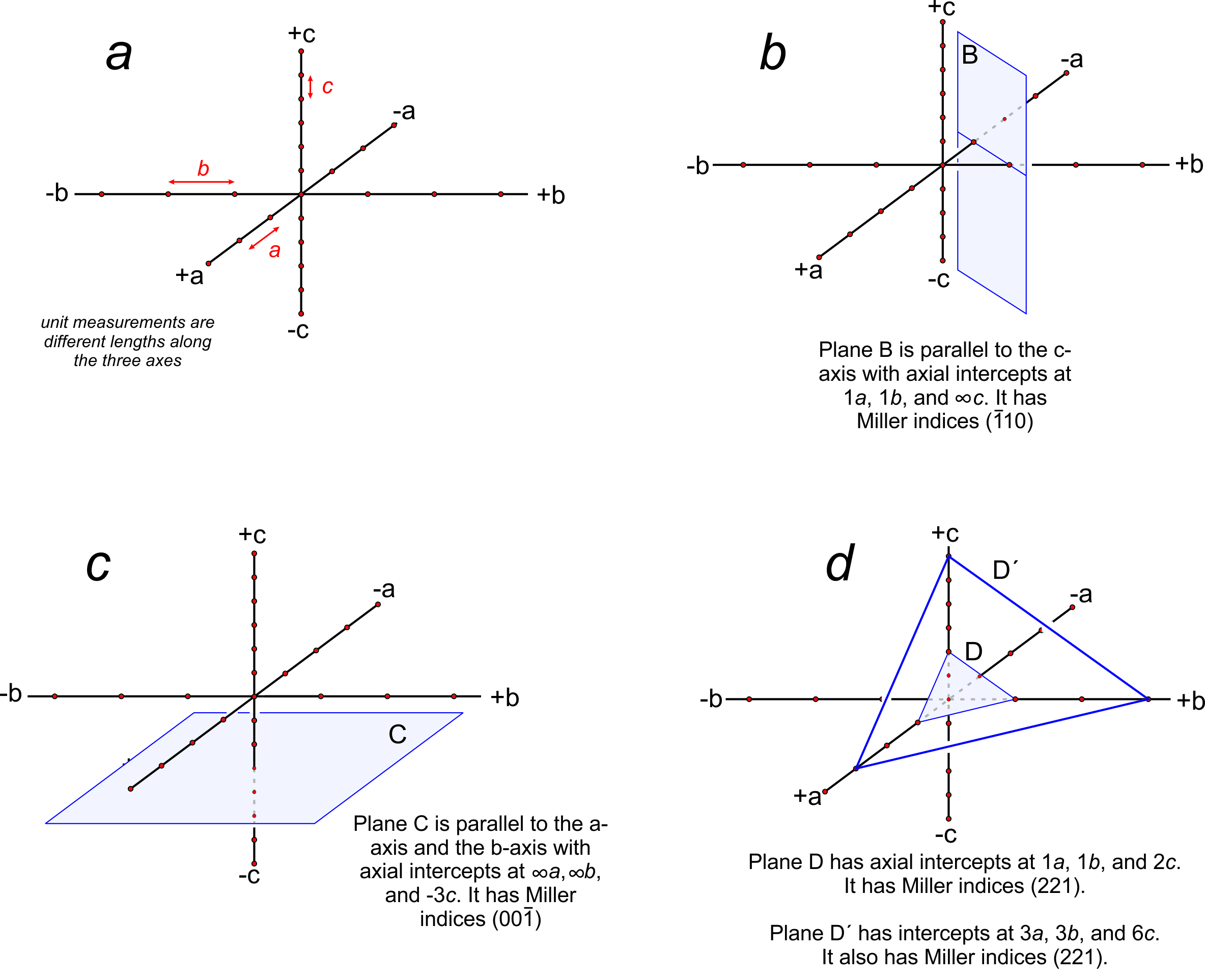
We can describe the orientation of a plane by listing its intercepts with the axes. For a face running parallel to an axis, the intercept is at ∞ (because the face never intersects the axis). In Figure 11.65b, the plane is parallel to the c-axis but intersects the a-axis and b-axis one unit from the origin. So, it has axial intercepts 1a, 1b, and ∞c, which we shorten to 1, 1, ∞. In Figure 11.65c, the plane is parallel to two axes and has axial intercepts ∞a, ∞b, 3c, or simply ∞, ∞, 3.
Crystal faces are commonly parallel to axes, but the use of ∞ to describe their orientations can be confusing and awkward. A second problem with using intercepts to describe face orientation is that parallel planes, such as plane D and plane D´ Figure 11.65d, have different intercepts. Crystallographers find this inconvenient because crystals may be large or small, but face orientation, not size, is generally the feature of greatest significance. To avoid these and other problems, crystallographers do not report axial intercepts. They use Miller indices instead.
11.9 Miller Indices
Miller indices were first developed in 1825 by W. Whewell, a professor of mineralogy at Cambridge University. We use them to describe the orientation of crystal faces, and also the orientations of cleavages and other planar properties. They are named after W. H. Miller, a student of Whewell’s, who promoted and popularized their use in 1839. The general symbol for a Miller index is (hkl), in which the letters h, k, and l each stand for an integer. Parentheses enclose the resulting Miller index. As with directions, bars above numbers show negative values and we do not include commas unless numbers have more than one digit.
We calculate Miller indices for a plane from its axial intercepts (Figure 11.65). The procedure is as follows:
·First, we invert axial intercept values. (∞ becomes zero after inversion.)
·Then we clear all fractions by multiplying by a constant.
·And we divide by a constant to eliminate common denominators (for primitive unit cells, but not for centered cells).
Consider the plane in Figure 11.65b. It has intercepts 1, 1, ∞. Inverting these values gives us (110), the Miller index of the plane. And the plane in Figure 11.65c has axial intercepts ∞, ∞, 3. Inverting these values gives us 0, 0, 1/3. Clearing the fraction gives us (001), the Miller index. We articulate it as “oh-oh-one.”
Figure 11.65d contains two planes. One has intercepts 1, 1, 2. The other has intercepts 3, 3, 6. Inverting intercepts for the first plane gives us 1, 1, 1/2. Clearing fractions yields the Miller index (221). Inverting intercepts for the second plane gives 1/3, 1/3, 1/6. Clearing fractions yields (221). So we see that parallel planes have the same Miller index. If the planes shown in this figure were crystal faces, we would call them the “two two one face” no matter their size or shape. Thus the Miller index describes the orientation of a crystal face with respect to crystallographic axes, but not the absolute size or location of the face. The relationship between planes and directions in a crystal depends on the crystal system. Except in the cubic system, the direction [uvw] is neither perpendicular nor parallel to planes with the Miller index (uvw).
Because crystal faces are parallel to rows of lattice points, they are parallel to planes that intercept crystal axes at an integral number of unit cells from the origin. Consequently, inversion of intercepts and clearing fractions always yields integers. This observation is known as the Law of Rational Indices. Another observational law, called Haüy’s Law:
blank■ Miller indices of faces generally contain low numbers.
For example, (111) is a common face in crystals, while (972) is not. Haüy’s law is really a corollary to the Law of Bravais, already discussed, which states that faces form parallel to planes of high lattice point density; planes with low values in their Miller index have the greatest lattice point density.
As mentioned previously, crystallographers have in the past used four axes for crystals in the hexagonal system. This yields a Miller index with four numbers (hkil). One of the first three values h, k, or i is redundant because we can always describe the location of a plane in three-dimensional space with three variables. In all cases: h + k + i = 0. Because of the redundancy, and to be consistent with other crystal systems, many crystallographers today use only three indices for hexagonal minerals.
For further discussion of Miller indices with examples, watch the videos linked here:
blank▶️ Video 11-5: Miller indices example (2 minutes)
blank▶️ Video 11-6: Miller indices of 0 (5 minutes)
blank▶️ Video 11-7: Miller indices for an octahedron (9 minutes)
blank▶️ Video 11-8: Miller indices for hexagonal minerals (4 minutes)
11.10 The Miller Indices of Planes within a Crystal Structure
We use Miller indices to describe the orientation of crystal faces, but we also use them to describe planes within a crystal structure. For example, we may be interested in knowing which planes in a unit cell contain the most atoms. For planes within a cell, we calculate Miller indices as we do for crystal faces, except that we do not clear common denominators after inversion of axial intercepts.
For example, if we calculate an index of (633) for a set of planes, we do not divide by 3 to give (211), as we do when calculating a Miller index for a crystal face. We do not do this because, besides orientation, the spacing and location of planes are important when we are talking about atomic arrangements and other aspects of crystal structures, and not talking about crystal faces.
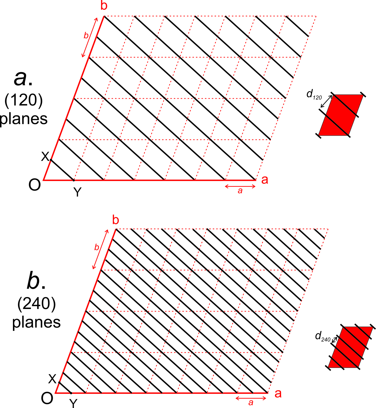
Figure 11.66a shows some two-dimensional unit cells cut perpendicular to the c-axis. The plane passing through points X and Y (and perpendicular to the page) has axial intercepts 1, 1/2, ∞, so its Miller index is (120). Because all unit cells are equivalent, we know identical (120) planes exist in all the unit cells.
Drawing a shows all equivalent (120) planes; when we discuss (120) planes within a crystal, we refer to this entire family, not just to one plane. As shown in the red inset drawing, four (120) planes intersect each unit cell. Two pass through the inside of the cell, and two through corners. Note that the axial intercepts of the (120) plane closest to the origin (O) are 1, 1/2, ∞, equivalent to 1/h, 1/k, 1/l for the entire family of planes. This relationship holds true for any family of (hkl) planes.
Different families of planes, with the same orientation but different spacings, have different indices. The drawings in Figure 11.66b show planes spaced half as far apart as the (120) planes; d240 = 1/2 d120. The plane closest to the origin has intercepts 1/2, 1/4, ∞. Inversion gives the Miller index (240). We do not clear the common denominator (divide by 2) because the families of (240) and (120) planes, although parallel, are not identical. There are twice as many (240) planes. The red inset drawing shows that seven (240) planes intersect each unit cell – two at opposite corners; the rest pass through the cell interior.
Because the Miller indices (120) and (240) are proportional, the two families of planes are parallel but the (240) planes are spaced apart half as much as the (120) planes. This is always the case – proportional indices mean planes are parallel and larger indices mean planes are closer together. If we are considering a set of planes that cause X-ray diffraction (discussed in detail in the next chapter), we describe them with Laue indices. These indices are the same as Miller indices for 1st-order diffraction, but we omit the parentheses. Thus we can have 120 or 240 diffraction, and the angle of diffraction is different because the two families of planes have different spacings. For 2nd-, 3rd-, or higher order diffraction (discussed in Chapter 12), Laue indices are twice, three-times, etc., the values of Miller indices.
11.11 Confusing Notations
As just discussed, crystallographers designate points, lines, and planes using different kinds of notations. The different notations, however, are somewhat similar, and this can be confusing. So, Box 11-5 summarizes the standard notations used, and gives examples.
● Box 11-5 Summary: Different Kinds of Crystallographic Notations
|
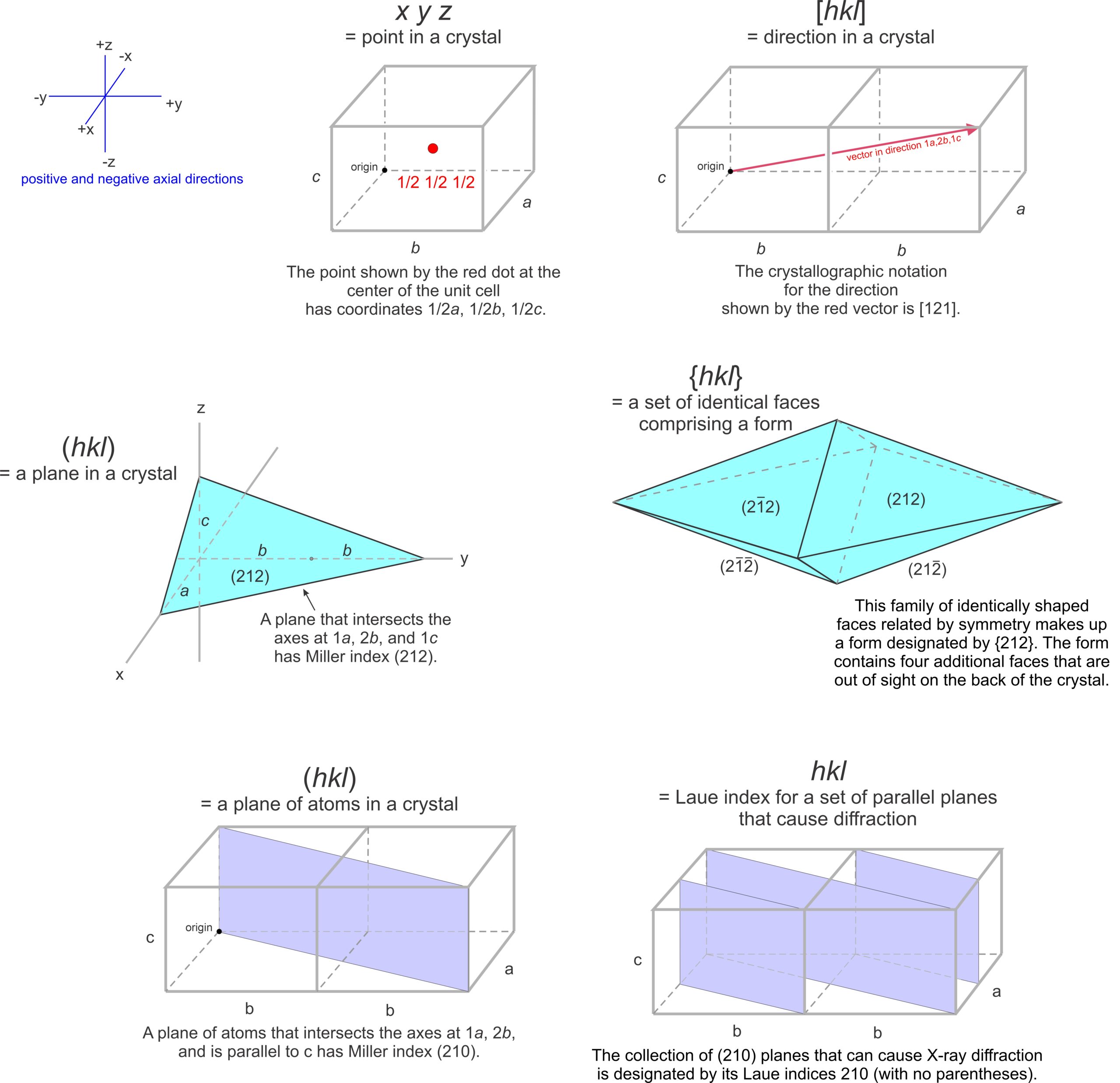
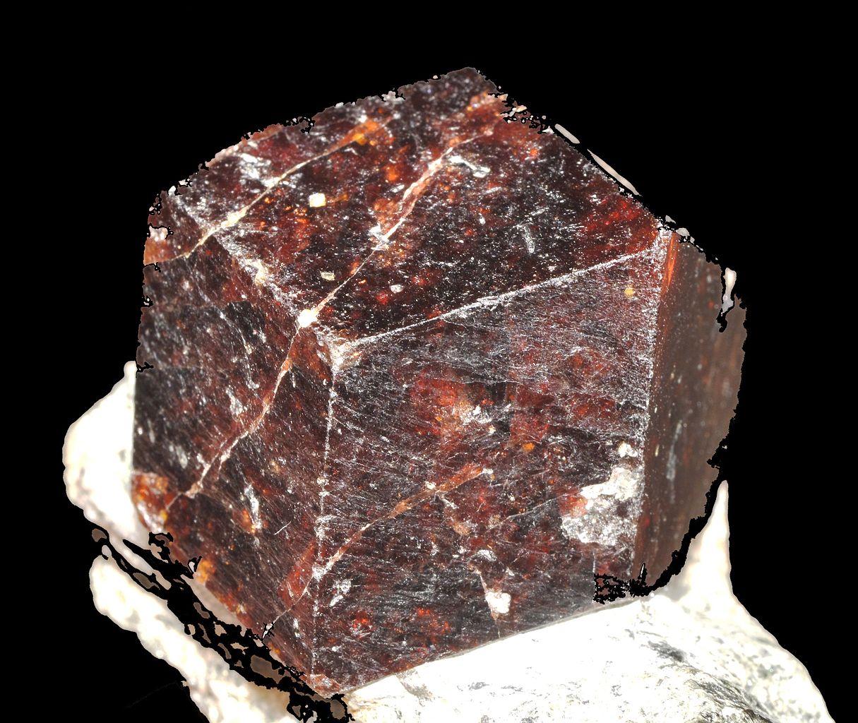
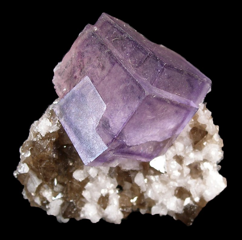
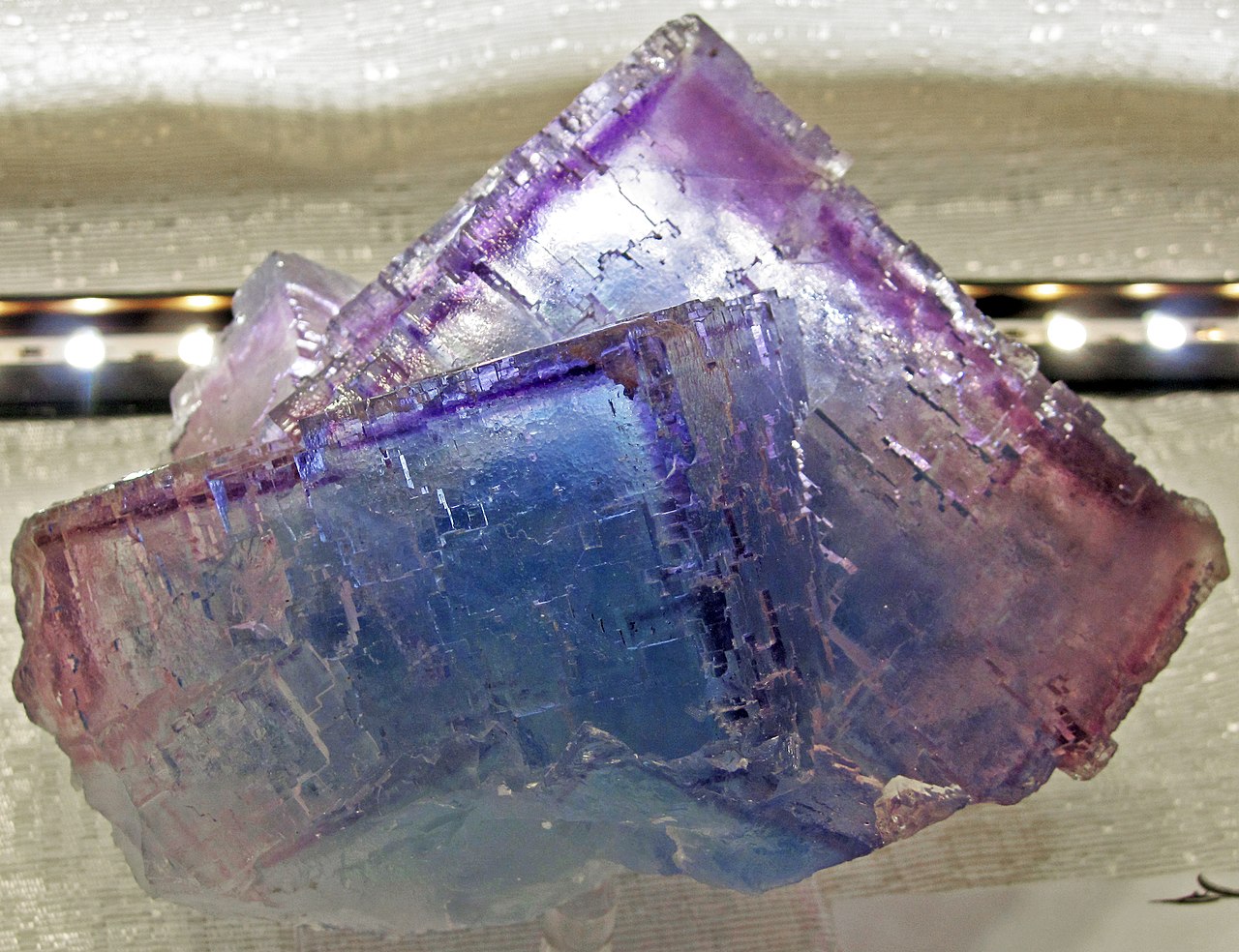
11.10 Crystal Forms and the Miller Index
The replacement of unknown or variable numbers in a Miller index with h, k, or l allows us to make generalizations. The index (hk0) describes the family of faces with their third index equal to zero. A Miller index including a zero describes a face is parallel to one or more axes (Figure 11.68a). The family of faces described by (hk0) is parallel to the c-axis; faces with the Miller index (00l) are parallel to both the a-axis and the b-axis.
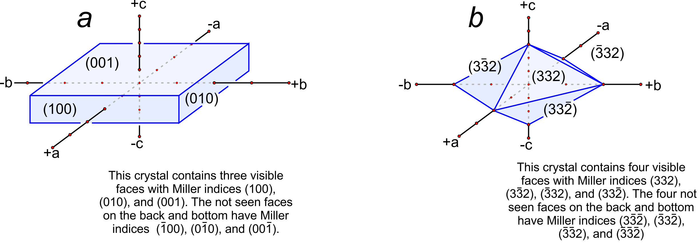
Figure 11.68a shows an orthorhombic prism with six faces. Some faces cannot be seen, but the Miller indices of all six are (100), (010), (001), (100), (010), and (001). Although this crystal contains three forms, indices for all faces contain the same numbers (two zeros and a one) but the order of numbers and the + or – sign changes.
Figure 11.68b shows an orthorhombic dipyramid. It contains only one form, and all the faces have the same numbers in their Miller index (332). This is always true for faces that belong to the same form; they always have similar Miller indices. This relationship is especially clear for crystals in the cubic system because high symmetry means that many forms may contain many identical faces.
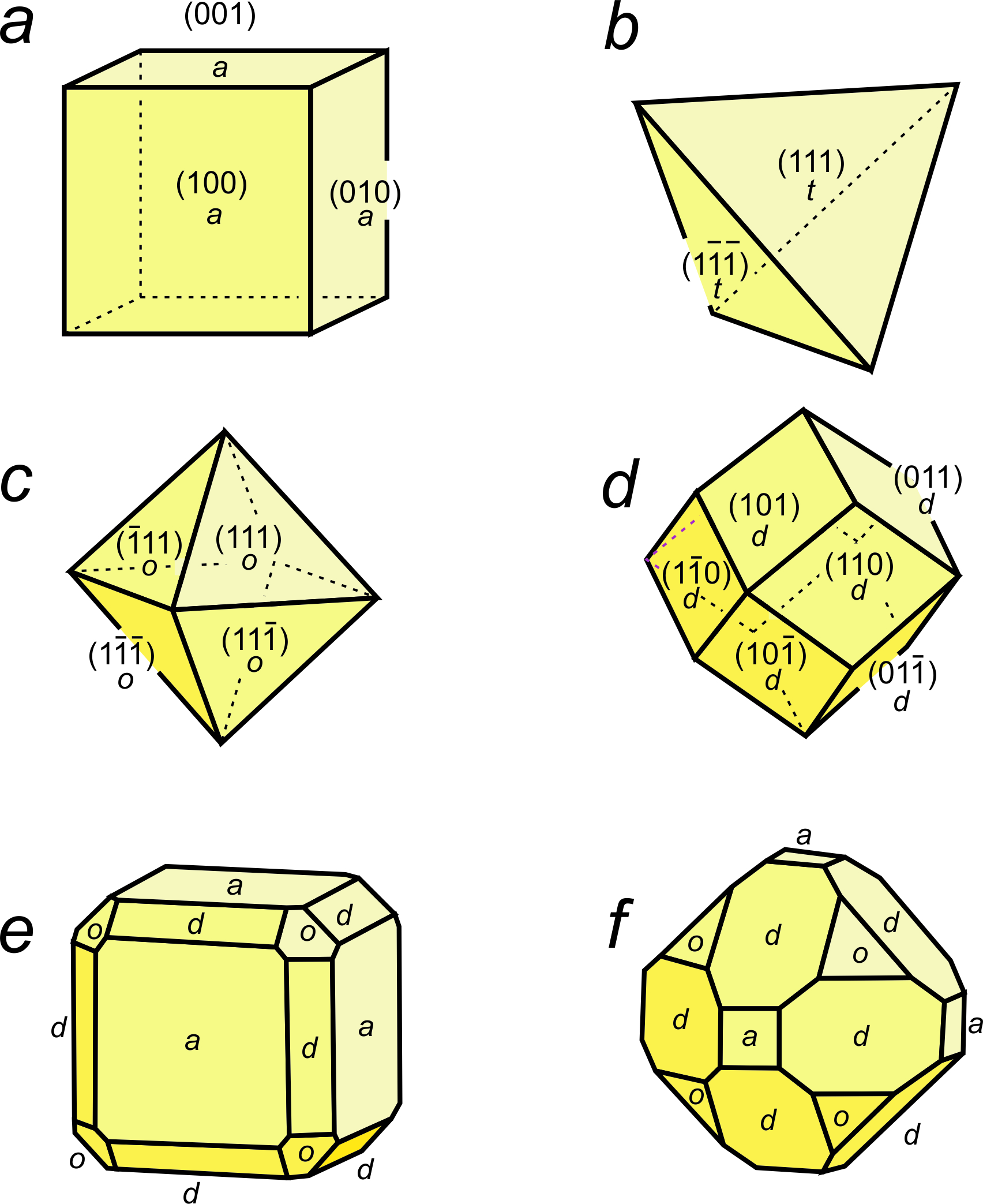
The six identical faces on the cube in Figure 11.69a have indices (001), (010), (100), (001), (010), and (100). We symbolize the entire form {100}, and the { } braces indicate the form contains all faces with the numerals 1, 0, and 0 in their Miller index, no matter the order.
The four faces on the tetrahedron in Figure 11.69b, and the eight faces on the octahedron in Figure 11.69c are all equilateral triangles. For both, the form is {111}. As Figure 11.69b and c demonstrate, two crystals of different shapes can have the same form if they belong to different point groups. The tetrahedron in Figure 11.69b belongs to point group 43m; the octahedron in Figure 11.69c belongs to point group 4/m32/m. If we know the point group and the form, we can calculate the orientation of faces. If a crystal contains only one form, we then know the shape of the crystal. Note that the cube, octahedron, and dodecahedron all belong to point group 4/m32/m. The cubic form is {100}, the octahedral form is {111}, and the dodecahedral form in Figure 11.69d is {110}.
Figure 11.69e shows a crystal containing three forms: cube {100}, octahedron {111}, and dodecahedron {110}. Because they all belong to point group 4/m32/m, we know the faces are oriented as shown. However, the crystal in Figure 11.69f belongs to the same point group and contains the same forms, but the size and shape of corresponding faces are different. We do not know the crystal shape if more than one form is present, unless we know some extra information.
Crystallographers sometimes label faces of the same form with the same letter as we have done in Figure 11.69. For some forms, the letter is just the first letter of the form name. For example, o indicates the octahedral form and d the dodecahedral form in the cubic system. Usually, however, the symbols are less obvious (we normally designate cube faces, for example, by the letter a); labels also vary from one crystal system to another.
11.10.1 Zones and Zone Axes
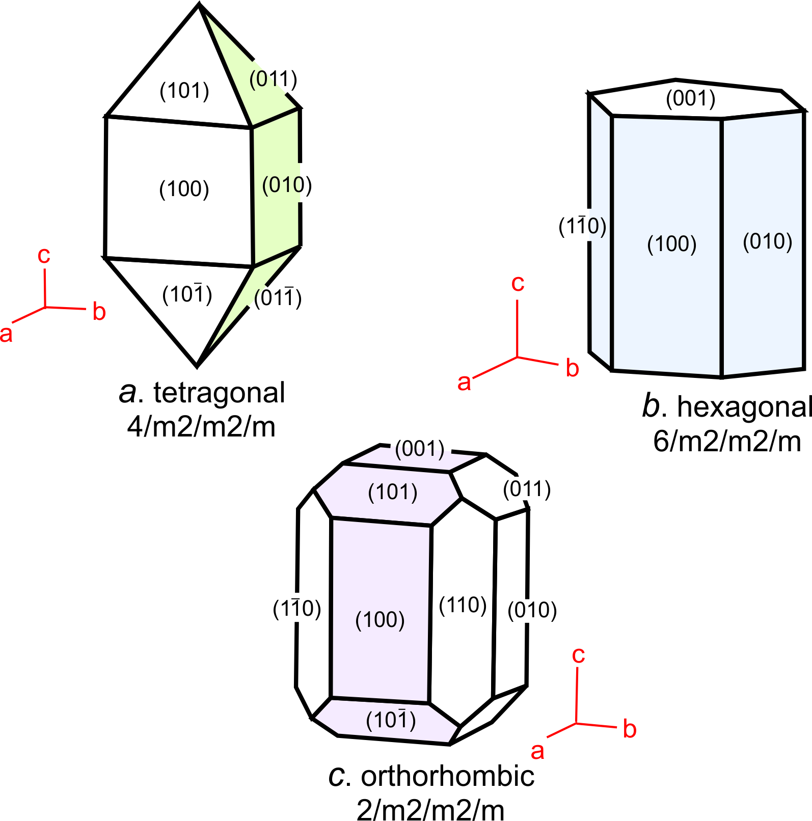
As discussed in Chapter 9, a set of faces parallel to a common direction defines a zone. We designate zones by the common direction, which we call the zone axis. Figure 11.70 shows examples of tetragonal, hexagonal, and orthorhombic crystals. The green faces in the tetragonal crystal (Figure 11.70a) form a zone. The faces are parallel to the a-axis. Three other faces (not visible) are also part of the zone. The zone axis is [100], parallel to a. Zones may contain faces from more than one form, as in this example.
Figure 11.70b shows a common zone in hexagonal minerals: 6 (blue) faces (three not seen) are parallel to the c-axis. The zone axis is [001]. And in Figure 11.70c, the zone (purple faces) comprises three forms and the zone axis is [010]. In all three drawings, additional zones are present besides those just mentioned. In these three examples, the zones axes have simple indices because they are parallel to crystal axes. Zones need not be parallel to axes, and consequently the indices may contain values other than 0 and 1.
11.10.2 General Forms and Special Forms
In any crystal class, a general form, which we generically designate {hkl}, contains faces that intersect the three crystal axes at different distances from the origin. In the cubic system, the Miller indices of the general form must all be different integers because unit cell dimensions are the same for all three axes (see Box 11-4.). For other systems, where some unit cell dimension are the same and some are different, two or more Miller indices may be the same. Thus, in the orthorhombic, monoclinic and triclinic systems the general form can be symbolized {hkl}, but {111} or {hhh} are also general forms. (We use three h’s in the symbol if we wish to show that all indices have the same integer value.) In the tetragonal system, the first two indices of the general form must be different since the a and b unit cell dimensions are the same. Thus, we may designate a tetragonal general form, for example, as {121} or {122}. In the hexagonal system, all three indices must be different and the general form is {hkl} or {123}, equivalent to any other form with three different Miller index values. In any crystal class, the general form contains the maximum number of faces that can be related by class symmetry.
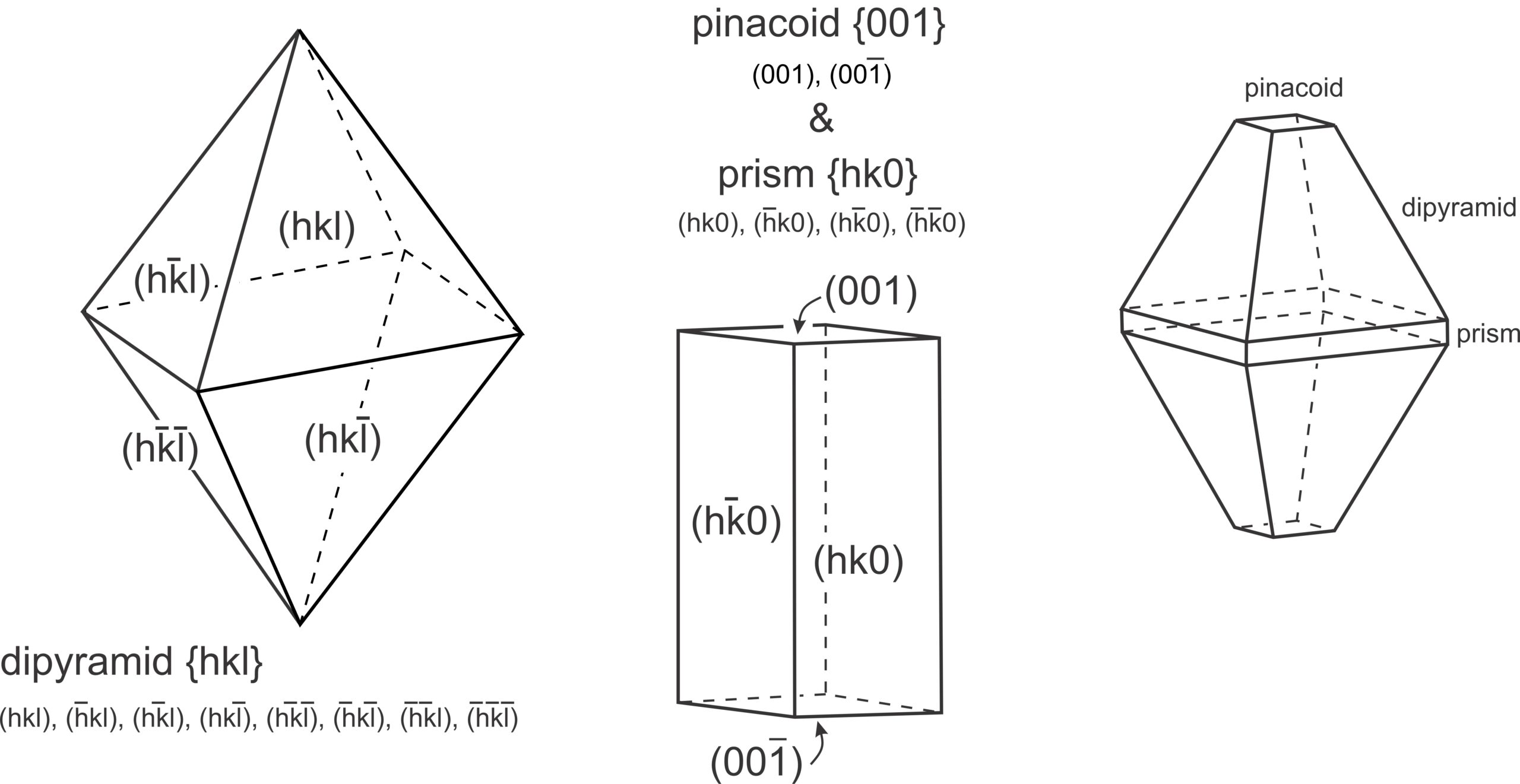
In contrast with general forms, special forms are parallel to one or two crystal axes. This means they are parallel or perpendicular to rotation axes or mirror planes. Consequently, special forms contain fewer faces than general forms for the same crystal class. For example, the drawing on the left in Figure 11.71 shows the general form for crystal class 2/m2/m2/m. It is an orthorhombic dipyramid. It contains eight faces, four of one shape and four of another. The middle drawing shows a crystal that contains six faces and two special forms, an orthorhombic pinacoid (top and bottom faces) and an orthorhombic prism (four vertical faces). The third crystal contains all three forms: the general form and the two special forms. All three crystals have the same symmetry.
● Box 11-6 General Forms, Special Forms, and Miller IndicesThe relationship between special forms and general forms is the same as the one between special points and general points discussed in the previous chapter. Faces of a general form are neither parallel nor perpendicular to any symmetry element, while faces of special forms are. Thus, in special forms, symmetry relates fewer equivalent faces. 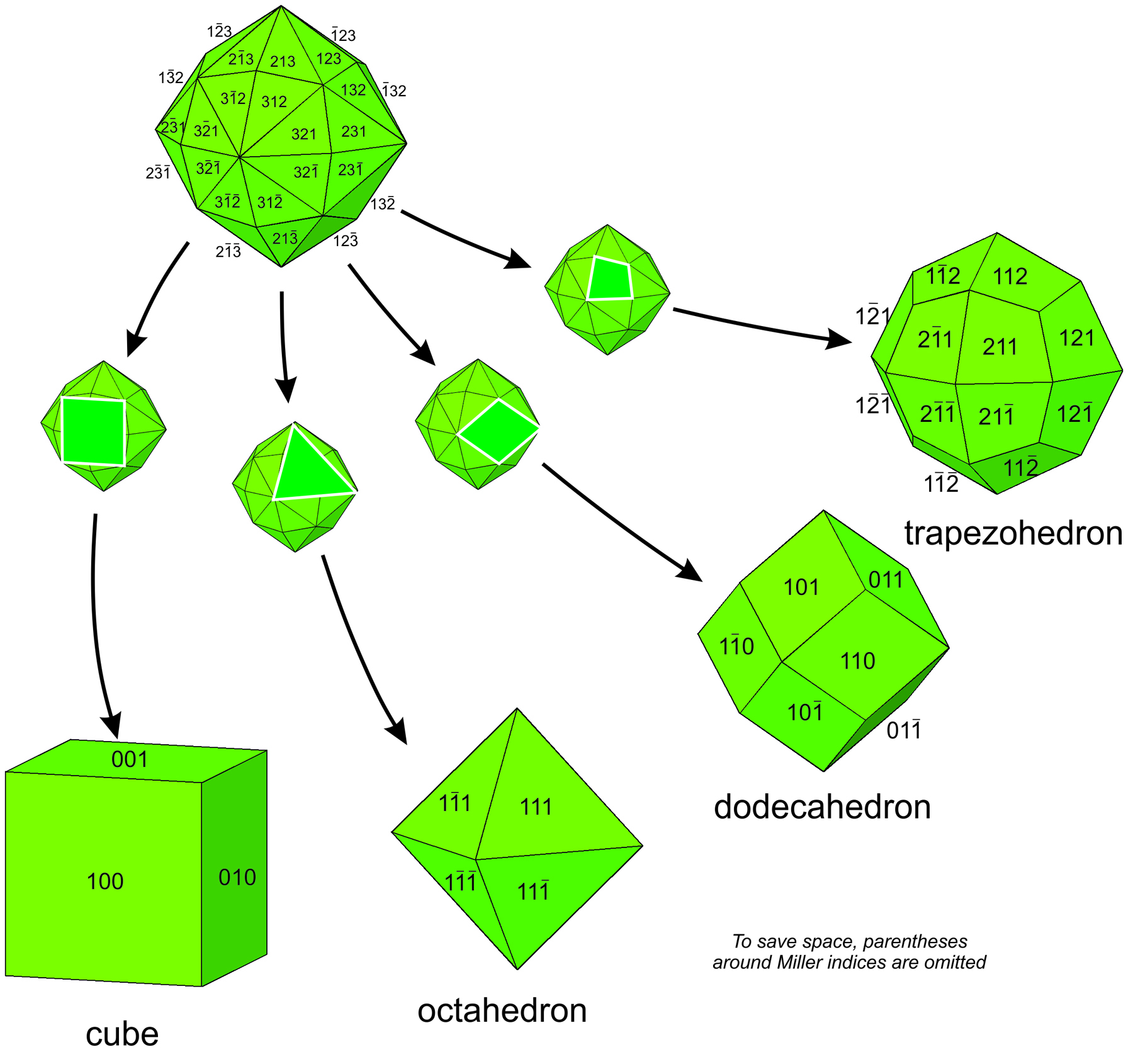 The hexoctahedron (Figure 11.72) is the general form in the 4/m32/m point group; its Miller index contains three different values. The simplest index is {123}, indicating that h ≠ k ≠ l and that none of the indices are zero. The hexoctahedron contains 48 triangular faces. We can think of this form as octahedron with each of its eight faces replaced by six smaller triangular faces; hence, its name. All other forms with the same symmetry are special forms in the hexoctahedral class. Crystals in this class may contain any of 15 forms singly or in combinations. Figure 11.72 shows four examples. See Box 10-3 and the table in Chapter 10 for other examples. In the cubic system, special forms have two or more identical indices in their Miller index, or have an index with value zero; Figure 11.72 contains examples. For example cube faces belong to the {h00} form; octahedron faces belong to the {hhh} form. The dodecahedron faces belong to the {hh0} form. Another related form, the trapezohedron, has Miller index {hkk}, signifying that two of its indices have the same value and that none are zero. h, k, and l can have any integer values and these relationships will hold. As shown in Figure 11.72, if we combine groups of faces on a hexoctahedron and replace them with a single face, we get a cube, octahedron, dodecahedron, or trapezohedron with no change in symmetry. Faces of the special forms all coincide with symmetry elements – that is what makes them special. Cube faces are perpendicular to 4-fold rotation axes, octahedron faces are perpendicular to 3-fold rotoinversion axes, dodecahedron faces are perpendicular to 2-fold axes, and trapezohedron faces are perpendicular to mirror planes. The examples seen in Figure 11.72 are all from a single point group, 4/m32/m. But the principles discussed apply to all 32 point groups. However, symmetry relationships and the nature of special forms are more difficult to see for some point groups, especially those with little symmetry. |
●Figure CreditsUncredited graphics/photos came from the authors and other primary contributors to this book. 11.1 Topaz from Pakistan, Didier Descouens, Wikimedia Commons Video 11-1: Bravais lattices, Keith Putirka, YouTube |

