12 Metamorphic Thermodynamics

KEY CONCEPTS

• Thermodynamics is the science that tells us which minerals or mineral assemblages will be stable under different conditions.
• The fundamental and most important thermodynamic variable is Gibbs free energy, abbreviated ΔG^O_f.
• The phase or phase assemblage with lowest Gibbs free energy is stable; but stable minerals or assemblages may change if conditions change because Gibbs free energies vary with pressure and temperature.
• The Gibbs free energy of a reaction (ΔG^O_rxn) is the sum of the Gibbs free energies of the reaction products, less the sum of the Gibbs free energies of the reactants. If ΔG^O_rxn is negative, the reaction proceeds to the right If positive, the reaction proceeds to the left.
• At high temperature, phases with high entropy are stable. At high pressure, phases with high density are stable.
• Reactions that do not involve any fluid phases generally plot as straight lines on phase diagrams. Reactions involving a gas or fluid phase (such as H₂O or CO₂) may plot as curves.
• Thermodynamic calculations can be complex and are most often facilitated by computer programs.
• If a mineral phase is diluted by other components, its reactivity decreases and its stability increases. So, reactions take place under different conditions depending on mineral composition.
• The minerals present in a metamorphic rock, and the compositions of those minerals, record the conditions at which equilibrium occurred.
• Some mineral reactions are very sensitive to temperature changes and, consequently, useful for estimating metamorphic temperature.
• Some mineral reactions are very sensitive to pressure changes and, consequently, useful for estimating metamorphic pressure.

12.1 Thermodynamics

The Oxford English Dictionary defines thermodynamics as “the theory of the relations between heat and mechanical energy, and of the conversion of either into the other.” In simpler terms, we can think of thermodynamics as the science that tells us which minerals or mineral assemblages will be stable under different conditions. In practical terms, thermodynamics allows us to predict what minerals will form at different conditions, a process we call forward modeling. Thermodynamics also allows us to use mineral assemblages and mineral compositions to determine the conditions at which a rock formed, a process we call thermobarometry.

Thermodynamics is especially well suited for analysis and interpretation of medium- to high-grade metamorphic rocks. This is because thermodynamics only applies to systems at equilibrium, and lower-temperature rocks often do not reach equilibrium. Sometimes, metamorphism overlaps with igneous processes. The thermodynamic properties of melts are complex, making thermodynamics more complicated for analyzing equilibria involving molten material. Nonetheless, the same principles apply.

12.1.1 Gibbs Free Energy: the Basis for Thermodynamic Calculations

All minerals, and other phases such as H₂O and CO₂, have an associated Gibbs free energy of formation value abbreviated ΔG^O_f. ΔG^O_f is the energy released or consumed when a pure phase is created from other phases.

Gibbs free energies are relative values, not absolute values. They allow us to compare energies, and thus the stabilities, of different phases but individual values by themselves have no significance. Because Gibbs Energy values are relative, we can arbitrarily assume some values to calculate others. So, by convention we assume the ΔG^O_f for any pure element is zero, and we calculate values for compounds relative to pure elements.

12.1.2 Equilibriums Involving Two Polymorphs

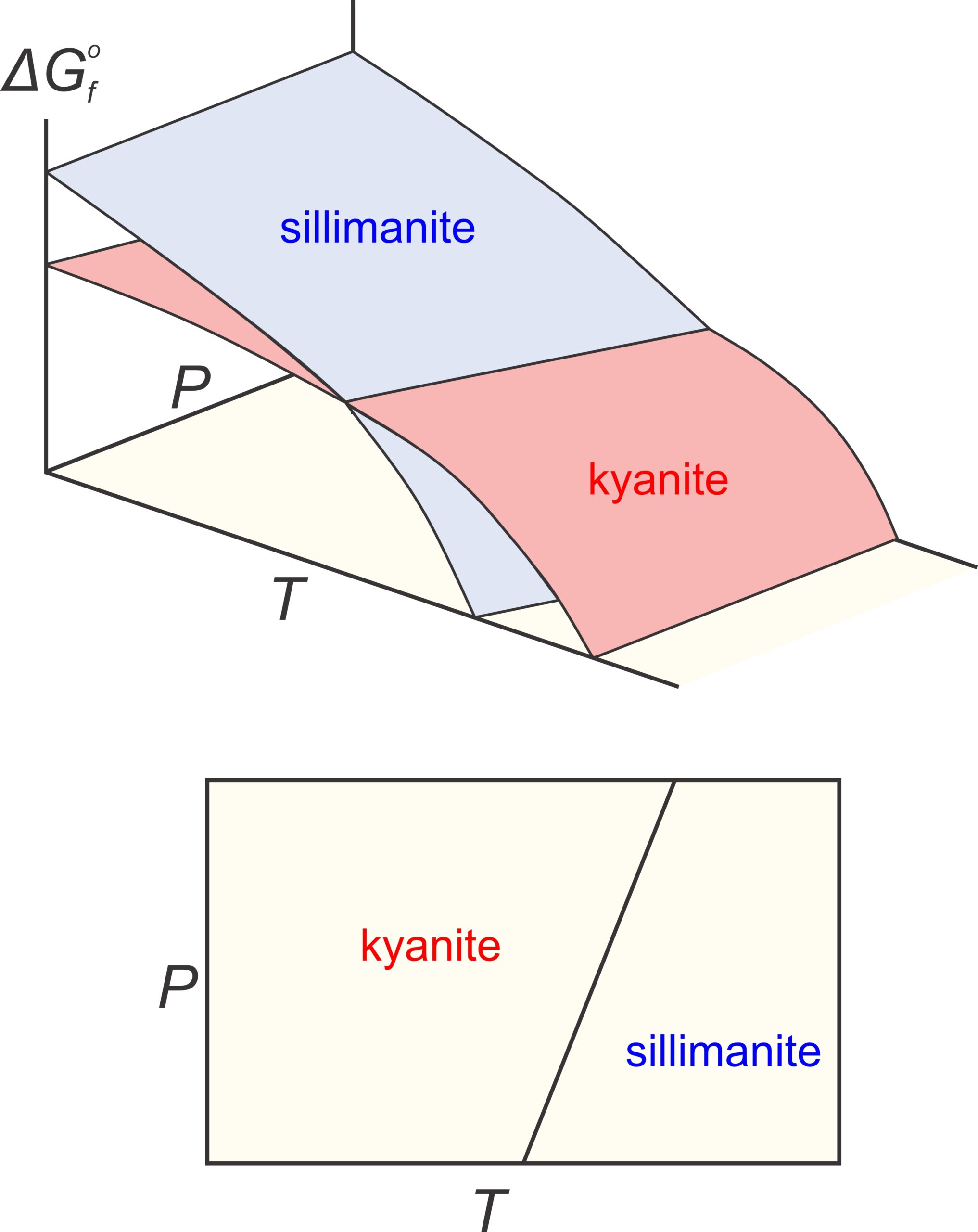
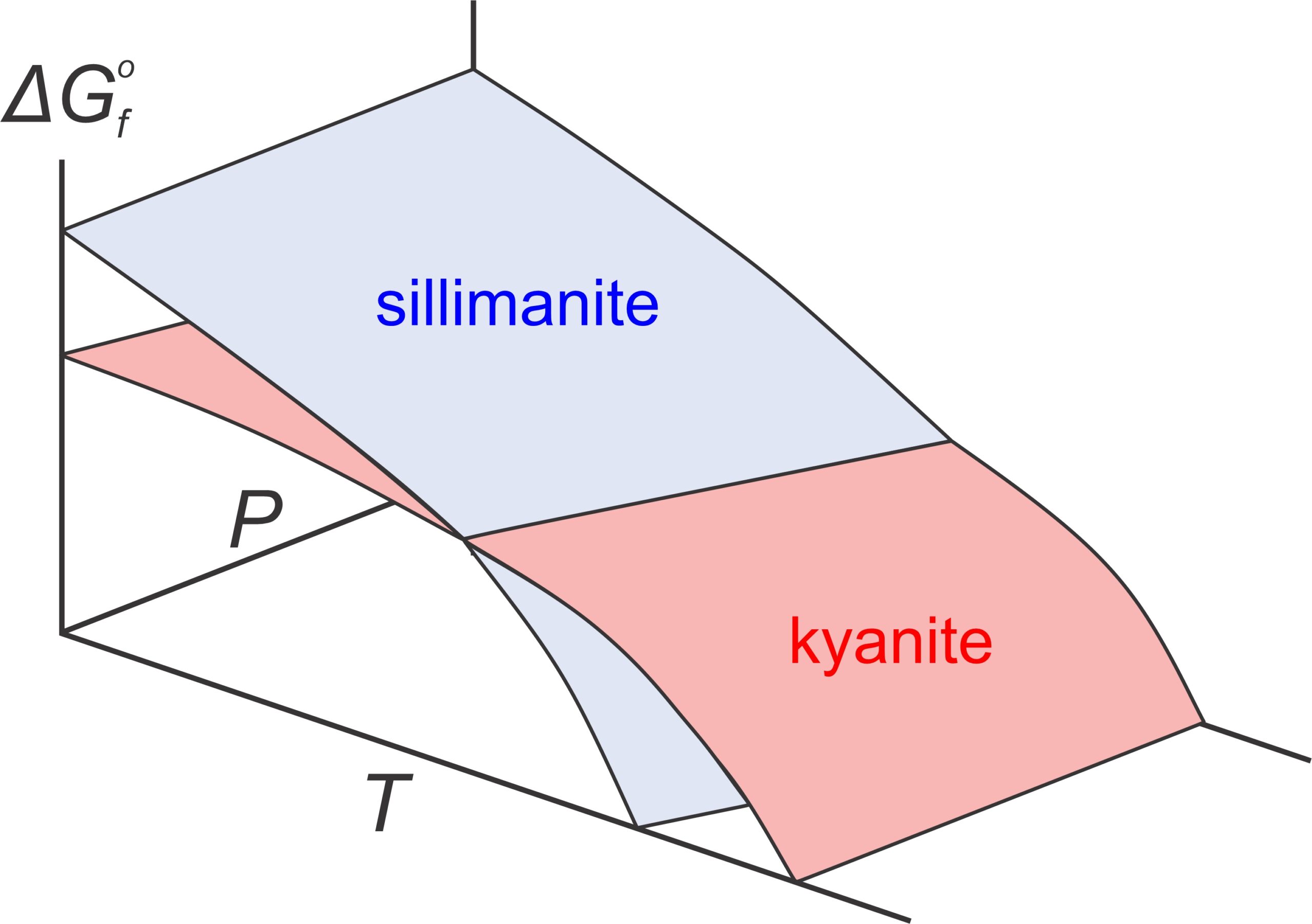
Consider the equilibrium between two Al₂SiO₅ polymorphs (kyanite and sillimanite). Both minerals have Gibbs free energy that varies with pressure and temperature, shown by the blue and red surfaces in the top part of Figure 12.1. At low temperature and high pressure, sillimanite (blue) has greater Gibbs free energy than kyanite (red). At higher temperature, and lower pressure, kyanite has greater Gibbs free energy than sillimanite. Because natural systems try to minimize energy, the polymorph with least energy is stable at different conditions. So, as reflected by the phase diagram (bottom of Figure 12.1), kyanite is stable at low temperature and elevated pressure, and sillimanite is stable at higher temperatures. Although it is not often evident, all P-T phase diagrams, like the one in Figure 12.1, are projections of Gibbs free energy surfaces onto a 2 dimensional pressure-temperature diagram. Lines in phase diagrams are P-T conditions at which energy surfaces intersect.

12.1.3 Gibbs Free Energy of a Reaction

Some reactions involve more than two phases. We can calculate the Gibbs free energy of any reaction (ΔG_rxn) by summing the Gibbs free energies of the right-hand side (products) of the reaction and subtracting the energies of the left-hand side (reactants). For example, consider a reaction involving three elements, which by assumption have Gibbs free energies of zero, reacting to form enstatite:

[Rxn 1]

Mg + Si + 3 O = enstatite Mg + Si + 3 O = MgSiO3

Reference books tell us that the Gibbs free energy of this reaction is -1,460.9 J/mole at room temperature and pressure. So, enstatite is 1,460.9 J/mol more stable than the elements separately. We say that -1,460.9 J/mole is the Gibbs free energy of formation of enstatite from elements at standard conditions. We symbolize this as ΔG^O_f (of enstatite). The degree superscript means we are talking about a pure phase, in this case pure (end member) enstatite, MgSiO₃. (Commonly, the degree superscript is not used unless the distinction between reactions of pure and impure phases needs to be distinguished.) We will see later that minerals in metamorphic reactions are often impure. (Enstatite, for example, usually contains some Fe replacing Mg.)

Sometimes, we may wish to consider the energy of formation of a mineral from oxides instead of from elements. For example, we can write the reaction:

[Rxn 2]

periclase + quartz = enstatite MgO + SiO2 = MgSiO3

The Gibbs free energy of this reaction, ΔG^O_f,oxides (of enstatite), is about -35.4 J/mole at room temperature and pressure.

The ΔG^O_f values given above for reactions 1 and 2 are both negative. So, enstatite is more stable than, and will form from, the separate elements or separate oxides at room temperature and pressure. Some energy produced as a reaction occurs may be given off as heat, and some may contribute to entropy. We will discuss entropy in more detail later.

12.1.4 Different Thermodynamic Variables

For any reaction, the Gibbs free energy of reaction (called the energy of reaction in the rest of this chapter) varies with pressure and temperature. The standard relationship is:

[Eqn 1]

ΔGrxn = ΔErxn + PΔVrxn – TΔSrxn

In Equation 1, P and T are pressure and temperature. They are intensive variables. which means they apply to an entire system and do not depend on the volume or content of the system being considered. ΔG_rxn, ΔE_rxn, ΔV_rxn, and ΔS_rxn are energy of reaction, internal energy, volume, and entropy of reaction, respectively. These are extensive variables, which means they vary depending on the composition and size (the extent) of the system being considered. They are molar quantities, so if more material is involved, we have greater changes in energy, internal energy, volume, and entropy as a reaction occurs.

We also define the enthalpy of a reaction (ΔH_rxn), another extensive variable:

[Eqn 2]

ΔHrxn = Erxn + PΔVrxn

and it follows from the above equations that:

[Eqn 3]

ΔGrxn = ΔHrxn – TΔSrxn

The different thermodynamic values tell us different things:

• If the energy of a reaction is negative (ΔG_rxn < 0), the reaction proceeds to the right if the system stays at thermodynamic equilibrium. If the energy of a reaction is positive (ΔG_rxn > 0), the reaction proceeds to the left if a system stays at thermodynamic equilibrium. If ΔG_rxn = 0, products and reactants are at equilibrium and P-T conditions fall on the reaction line on a phase diagram.

• The volume of a reaction (ΔV_rxn), calculated as the volume of the phases on the right-hand side of the reaction minus the volume of the phases on the left, tells us whether the products or the reactants of a reaction have greater volume. If ΔV_rxn >0, the right-hand side of the reaction has greater volume and is stable at lower pressure than the left-hand side. If ΔV_rxn <0, the opposite is true.

• The entropy of a reaction (ΔS_rxn), calculated as the entropy of the phases on the right-hand side of the reaction minus the entropy of the phases on the left, tells us whether the products or reactants are more disordered. For example, the reaction of liquid water to steam (boiling) has a large associated increase in entropy. The steam molecules are more dispersed, are less well bonded together, and have greater kinetic energy. If ΔS_rxn >0, the right-hand side of the reaction has greater entropy and is stable at higher temperature than the left-hand side. If ΔS_rxn <0, the opposite is true.

• The enthalpy of reaction (ΔH_rxn), calculated as the enthalpy of the phases on the right-hand side of the reaction minus the enthalpy of phases on the left, tells us how much heat will flow in or out of the system during reaction. If ΔH_rxn < 0, the reaction is exothermic – it releases heat. For example, combustion of carbon-based compounds (C + O₂ = CO₂) gives off a lot of heat. If ΔH_rxn > 0, the reaction is endothermic – it consumes heat. Melting ice by the reaction H₂O (ice) = H₂O (water), is endothermic and, consequently, cools our gin and tonics in the summer.

● Box 12.1 Thermodynamic Units and Conversion Factors ΔGrxn – The units for ΔGrxn are J/mol or cal/mol. ΔHrxn – The units for ΔHrxn are J/mol or cal/mol. ΔSrxn – The units for ΔSrxn are J/K-mol or cal/deg-mol. ΔVrxn – The units for ΔVrxn are cm3/mol or, less commonly J/bar/mol. The International System of Units, abbreviated as the SI system, which is the most widely used system, expresses energy in joules (J) and temperature in Kelvin (K). In the SI system, 1 J = 1 N m (1 newton meter). Sometimes, however, energy is given in calories. 1 calorie is the heat required to raise the temperature of 1 g of pure water by 1°C at 1 atm pressure. Additionally, when doing thermodynamic calculations, energy may come out to be in units of cm3•bar. The following conversion factor help convert between different units: xxx1 cal = 4.184 J xxx1 J/bar = 10 cm3 xxx1 cal/bar = 41.84 cm3 xxx0 oC = 273 K

12.1.5 Variations in Gibbs Free Energy with P and T

[Eqn 1]

ΔGrxn = ΔErxn + PΔVrxn – TΔSrxn

Look closely at Equation 1 describing the energy of a reaction. The right-hand side contains three terms. The first is the change in internal energy – a constant that varies depending on the phases involved. The second is a PV term that equates Gibbs Energy with volume and pressure. More voluminous phases have greater Gibbs free energy because of this term. (Recall that the energy of an ideal gas is proportional to volume because, according to the Ideal Gas Law, energy = PV = nRT.) The third term involves entropy (S). Entropy is a measure of disorder. Some phases can absorb energy simply by becoming disordered. Temperature may not increase, volume may remain the same, but energy disappears.

If a system is at equilibrium, phases with lower Gibbs free energy are more stable than phases with higher Gibbs free energy. So, at high temperature, phases with high entropy are very stable – the TS term in Equation 1 becomes dominant and the TS term has a negative sign, thus lowering Gibbs free energy. Similarly, at high pressure, phases with high volume are unstable. The PV term has a high positive value, making the voluminous phase unstable. (Although your intuition may not work well when considering entropy, it should seem reasonable that dense phases are more stable at high pressure than phases of less density.)

Consider the reaction:

[Rxn 3]

albite = jadeite + quartz NaAlSi3O8 = NaAlSi2O6 + SiO2

ΔG^O_f values vary, but at any specific pressure and temperature:

[Eqn 4]

ΔGrxn,P,T = ΔGOf(jadeite) + ΔGOf (quartz) – ΔGOf(albite)

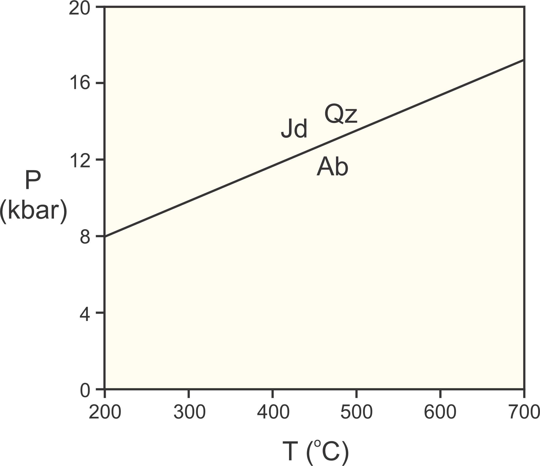
Under Earth surface conditions, the energy of this reaction is greater than zero. Consequently, albite is stable and the assemblage jadeite + quartz is unstable. But, at higher pressures, things turn around, and jadeite + quartz has lower Gibbs free energy, and is more stable than albite. Figure 12.2 depicts these relationships. Jadeite and quartz have lower volume than albite, and so are stable at high pressure. Albite has greater entropy than jadeite and quartz, and so is stable on the high-temperature side of the reaction.

 

12.1.6 Calculating the Location of a Reaction

No matter the conditions, if a reaction is at equilibrium, the energy of reaction is 0. So, following equation 1 above, at equilibrium:

[Eqn 5]

0 = ΔGrxn = ΔErxn + PΔVrxn –TΔSrxn

Because ΔE_rxn is a constant, Equation 5 suggests this equation is linear with P and T. Consequently, we might expect all reaction to plot as straight lines on P-T diagrams. However, the volume and entropy of phases (and therefore the volume and entropies of reactions) vary somewhat with pressure and temperature and reactions may curve on P-T diagrams. Still, most reactions that do not involve vapor phases such as H₂O or CO₂, plot as near straight lines on P-T diagrams and examination of Equation 5 tells us that the slope of a reaction is:

[Eqn 6]

dP/dT = ΔSrxn/ΔVrxn

This is the Clapeyron equation (also called the Clausius-Clapeyron equation). This equation states that the slope (rise/run) of a univariant reaction plotted on a P-T diagram is equal to the entropy change (ΔS_rxn) of the reaction divided by the volume change (ΔV_rxn) of the reaction. The Clapeyron equation only tells us the slope of a reaction line, not the position of the reaction in pressure-temperature space. We must do further thermodynamic calculations or use experimental data to determine the actual position.

Most solid-solid reactions plot on a P-T diagram as essentially straight lines because ΔS_rxn and ΔV_rxn do not change much with varying pressure or temperature. To the extent that ΔS_rxn and ΔV_rxn do change, the changes are about proportional, also explaining the straight line geometry.

For reactions involving a gas or fluid phase (such as H₂O or CO₂), ΔS_rxn and ΔV_rxn may vary significantly with pressure and temperature, because of increasing entropy as a fluid is produced, and because of the extreme compressibility of fluids. This is why reactions involving H₂O and CO₂ curve on P-T diagrams as pressure approaches zero. We saw examples in the previous chapter. Many reactions involving H₂O or CO₂, however, plot as near straight lines at elevated pressure where gas properties vary more linearly with P and T.

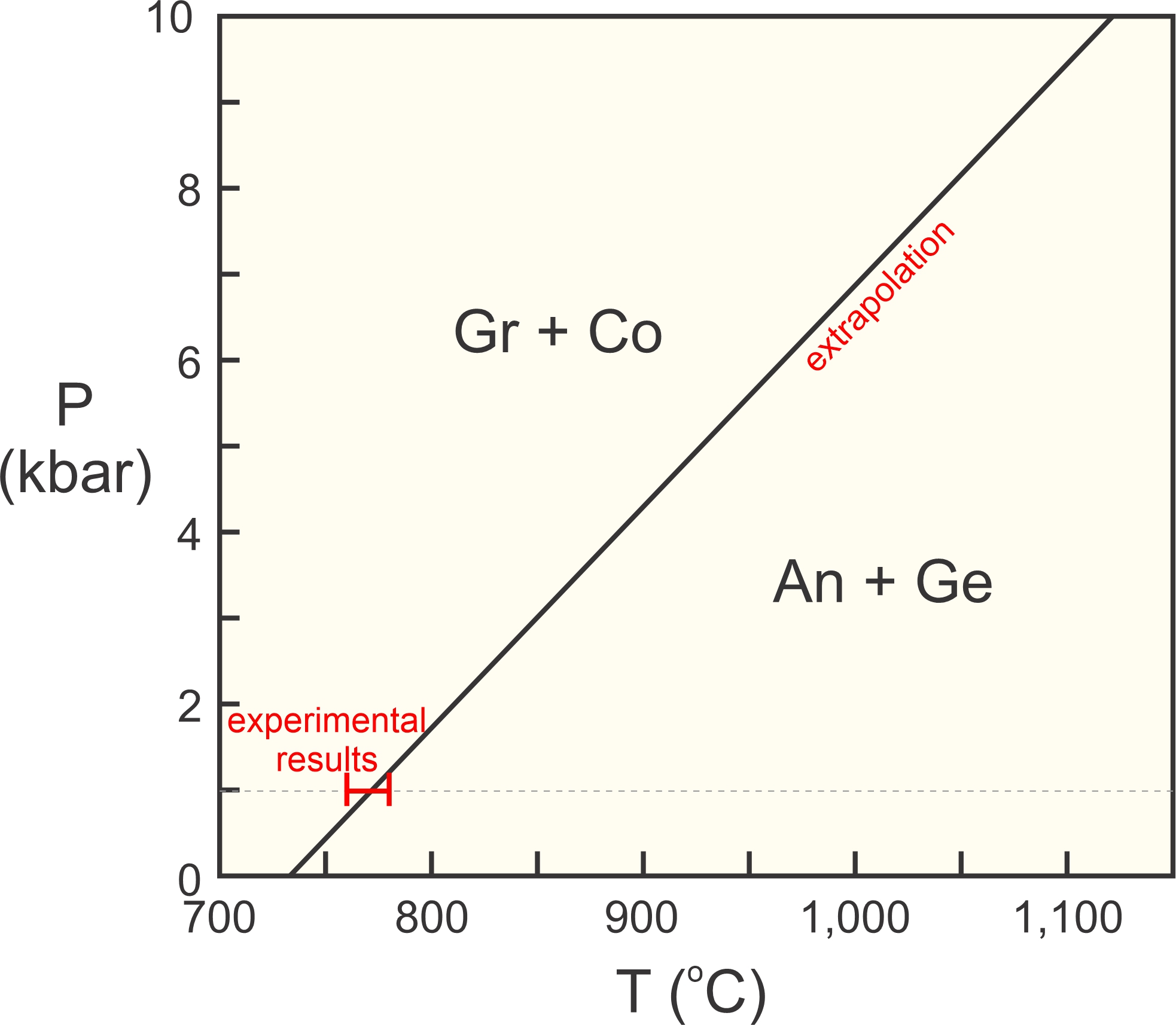
For an example of application of the Clapeyron equation, consider the reaction between grossular (Gr), corundum (Co), anorthite (An) and gehlenite (Ge):

[Rxn 4]

Gr + Co = An + Ge Ca3Al2Si3O12 + Al2O3 = CaAl2Si2O8 + Ca2Al2SiO7

In an experimental study, Boettcher (1970) found that this reaction takes place between 760 and 780 °C at 1 kbar pressure. We can use Boettcher’s results and extrapolate this reaction to higher pressures. This is a solid-solid reaction, so assuming that ΔS/ΔV of reaction is about constant is reasonable. This means the reaction will plot as a straight line on a P-T diagram. Thus we can calculate the slope of the reaction at 1 bar and use that to extrapolate.

From thermodynamic reference books, we find the following room temperature-pressure molar entropy and volume values for the four phases involved:

Table 12.1. Thermodynamic Data
mineral	S (J/K)	V (cm3)
anorthite (An)	199.3	100.79
gehlenite (Ge)	209.8	90.24
grossular (Gr)	255.5	125.3
corundum (Co)	50.92	25.575

So, for Reaction 4:

ΔV = V_An + V_Ge – V_Gr – V_Co = 100.79 + 90.24 – 125.3 – 25.575 = -40.155 cm³/mol
ΔS = S_An + S_Ge – S_Gr – S_Co = 199.3 + 209.8 – 255.5 – 50.92 = -102.68 J/K-mol

Now, we can use the Clapeyron equation to calculate the reaction slope:

dP/dT = ΔS/ΔV
= (10 cm³-bar/J) x (-102.68 J/K-mol) / (-40.155 cm³/mol)
= 25.57 bar/degK

Note the conversion factor (10 cm³-bar/J) in this calculation that makes all units the same.

Using the slope of 25.57 bar/deg, we find that if the reaction takes place at 770 °C at 1 Kbar, it must take place at 1,121 °C at 10 Kbar. We can plot it on a P-T phase diagram, as shown in Figure 12.3.

The example above shows how we can use experimental results and the Clapeyron equation to extrapolate reactions to conditions outside the experimental range. Without experimental data, however, we can calculate the location of reactions on a phase diagram entirely from thermodynamic data.

Enthalpies of many minerals have been determined using calorimetry, and entropies have been calculated based on a different kind of calorimetry. So, there are many quite robust thermodynamic databases available for use. A problem, however, is that values determined from calorimetry, especially enthalpy values, sometimes have large uncertainties. To overcome the uncertainties and determine the “best” values to use, petrologists have derived internally consistent thermodynamic databases that reproduce the results of many different experimental studies.

Thermodynamic calculations can be complex, even with a reliable database. Doing the calculations by hand can be impossible or, at best, incredibly time consuming. In part this is because mineral volume and entropy vary with pressure and temperature. This is a minor consideration for many solid-solid reactions, but not for all. Additionally, the properties of H₂O, CO₂, or any fluid phase, vary in complicated ways with pressure and temperature. Consequently, petrologists today use computer programs that consider all the complications.

12.2 Thermodynamic Modeling Programs

Thermodynamic modeling programs fall into several categories. Some simply calculate phase diagrams. For example, most of the phase diagrams seen in this book were derived using the program TWQ, created by Rob Berman at the Canadian Geological Survey about 30 years ago. TWQ is quite easy to use and highly recommended.

A second, and very popular, type of modeling program creates pseudosections that show stable mineral assemblages for a given bulk-rock composition at different P-T conditions. The most widely used of these are Thermocalc, Perple_X, and Theriak-Domino. These programs are significantly more complicated than TWQ.

A third kind of modeling program calculates phase equilibria for systems including a melt. And a number of programs are available for calculating equilibria involving aqueous species. More complicated programs involving solid and melt equilibria are also available, but most have a narrower focus than the programs listed above.

Lanari and Duesterhoeft (2019) provide a nice review of the standard approaches used for modeling and the thermodynamic background . Their article also compares some of the differences between the various programs. Other review information can be found in the proceedings of the 2021 International Phase Equilibrium Modeling E-workshop. Powerpoint and pdf files from the workshop contain many useful links. Comparisons and descriptions are also available on SERC’s Teaching Phase Equilibria/Advanced Modeling Programs page. Box 12.2 contains links to all of these and to homepages where different modeling programs my be downloaded.

● Box 12.2 Useful Links: Thermodynamic Modeling Programs ▪P. Lanari, E. Duesterhoeft (2019) Modeling Metamorphic Rocks Using Equilibrium Thermodynamics and Internally Consistent Databases: Past Achievements, Problems and Perspectives ▪Proceedings of the International Phase Equilibrium Modeling e-workshop, May 10-14, 2021 ▪SERC’s Teaching Phase Equilibria/Advanced Modeling Programs page ▪winTWQ homepage ▪Perple_X homepage ▪Thermocalc homepage ▪Theriak-Domino homepage

blank

12.3 Impure Minerals

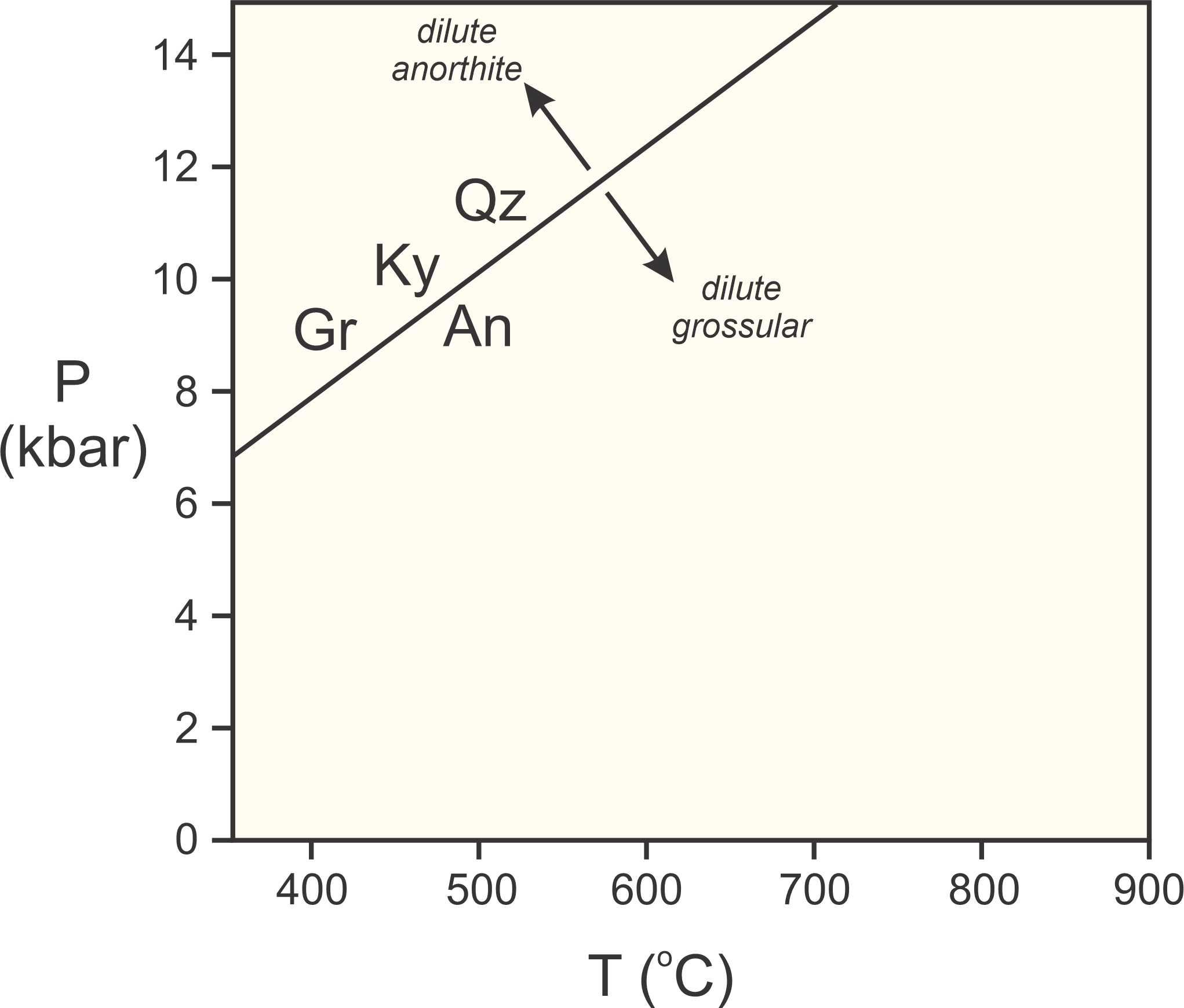
Many minerals are impure; they are solid solutions composed of multiple end members. Consider for example this reaction involving grossular (Gr), kyanite (Ky), quartz (Qz), and anorthite (An):

[Rxn 5]

grossular + 2 kyanite + quartz = 3 anorthite Ca3Al2Si3O12 + 2 Al2SiO5 + SiO2 = 3 CaAl2Si2O8

Figure 12.4 shows where this reaction occurs in P-T space if all minerals are pure end members. Kyanite and quartz vary little in composition, generally being very close to end member Al₂SiO₅ and SiO₂. However, in most metamorphic rocks (especially rocks that contain grossular, kyanite, and quartz) grossular and anorthite are part of garnet and plagioclase solid solutions.

When minerals are diluted, it decreases their reactivity and extends their stability. So, if anorthite is diluted because it is a component in plagioclase, Reaction 5 moves to higher pressure. Similarly, grossular is usually a minor component in garnet, so its reactivity is much less than it would be if pure. This pushes the reaction to lower pressure. Consequently, Reaction 5 may take place in a metamorphic rock, but does not take place at the same P-T conditions that it would if the minerals were had end-member compositions (sh0wn by arrows in Figure 12.4)

We use the term activity, and the variable a, to describe the reactivity of an end member in a solid solution mineral. The activity of a pure end member is 1. If none of the end-member is present, its activity is 0. Suppose we have plagioclase that is 100% anorthite. Then, the activity of anorthite, a_An = 1. If we add albite or orthoclase to the feldspar, anorthite becomes diluted and its activity decreases. If a feldspar contains no anorthite, the activity of anorthite is zero. So, activities can range from 1 to 0.

Raoult’s law, promulgated by French chemist François-Marie Raoult in 1887, says that the reactivity (activity) of an ideal gas in a gas mixture is equal to its mole fraction. Some mineral solutions are close to ideal, too, and we can often approximate activity as being equal to mole fraction without introducing large errors. So, for example, if a feldspar is 30% anorthite, the activity of anorthite is about 0.3. For the most accurate calculations, however, petrologists use computer programs that include complicated models that calculate activities from mineral compositions. For a brief introduction to activity models go to Activity Models at https://serc.carleton.edu/research_education/equilibria/activitymodels.html. For a more in-depth discussion, go to the 2019 paper by Lanari and Duesterhoeft at https://doi.org/10.1093/petrology/egy105.

12.3.1 Calculations Involving Equilibrium Constants

12.3.1.1 Net-Transfer Reactions

For a reaction involving impure minerals, we define the equilibrium constant (K) as the product of the activities of the products on the right-hand side of the reaction divided by the product of the activities of the reactants on the left-hand side. So, for Reaction 5, we calculate the equilibrium constant using Equation 7, below:

[Rxn 5]

grossular + 2 kyanite + quartz = 3 anorthite Ca3Al2Si3O12 + 2 Al2SiO5 + SiO2 = 3 CaAl2Si2O8

[Eqn 7]

K = a3An  / aGr a2Ky aQz

The exponents on the activity terms for kyanite and anorthite are because the reaction involves 3 moles of anorthite and 2 moles of kyanite. However, kyanite and quartz, as pointed out above, are generally pure Al₂SiO₅ and SiO₂, so their activities = 1. The above equation then becomes:

[Eqn 8]

K = a3An  / aGr

Consider pure phases. ΔG^O_f is the energy of reaction when all phases are pure – when all have activities of 1:

[Eqn 9]

ΔGOrxn = ΔEOrxn + PΔVOrxn – TΔSOrxn

The degree symbols remind us that the thermodynamic values are for pure phases. For reactions involving impure phases:

[Eqn 10]

ΔGrxn = ΔGOrxn + RT ln (K)

In Equation 10, R is the gas constant, and temperature (T) is in Kelvin. The ΔG_rxn term to the left of the equal sign does not have a degree superscript because it is the energy of reaction for impure phases.

At equilibrium (along a reaction line), the energy of reaction is 0:

[Eqn 11]

0 = ΔGrxn = ΔGOrxn + RT ln (K)

So, combining Equation 11 with Equation 9, for any reaction, we get:

[Eqn 12]

0 = ΔGOrxn = ΔEOrxn + PΔVOrxn – TΔSOrxn+ RT ln (a3An / aGr )

Note that if all phases are pure end-members, all activities equal 1. The equilibrium constant (K) is therefore 1 and its log is zero, so the RT ln (K) term goes away.

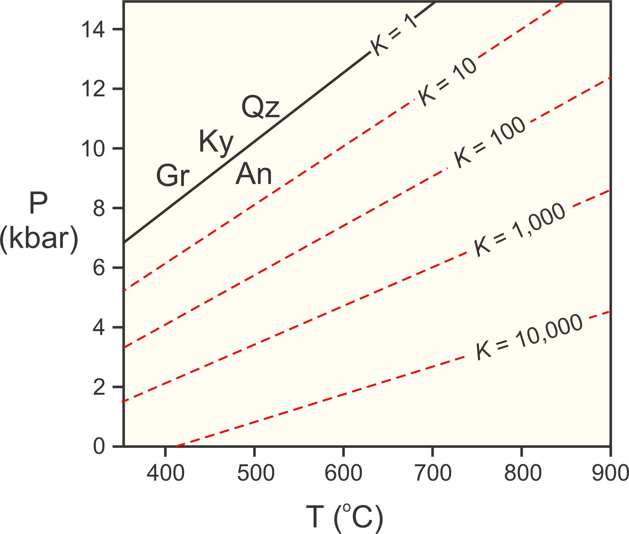
Figure 12.5 shows end-member Reaction 5, occurring at the same P-T conditions as in Figure 12.4 (black line). The figure also shows where the reaction occurs for various values of the equilibrium constant K (red dashed lines). Natural garnet always contain some grossular, and natural plagioclase always contains some anorthite. But garnet and plagioclase are never pure grossular and anorthite, and the equilibrium constant for Reaction 5 (calculated using Equation 8) is always greater than one. This means that rocks containing garnet, kyanite, quartz, and plagioclase equilibrated at lower pressure than where the end-member reaction occurs.

If a rock contains garnet, kyanite, quartz, and plagioclase, and if we know the compositions of the garnet and plagioclase, we can calculate the equilibrium constant using Equation 8. We then can use a diagram such as the one in Figure 12.5 to find a line describing the P-T conditions at which the rock may have equilibrated. This is the basis for what is called the GASP geobarometer. The acronym GASP stands for garnet-aluminosilicate-silica-plagioclase.

12.3.1.2 What About Exchange Reactions?

The example just examined above was for a net-transfer reaction. Now, let’s consider an exchange reaction:

[Rxn 6]

Fe-garnet + Mg-biotite = Mg-garnet + Fe-biotite

For this reaction, and other exchange reactions, we define a distribution coefficient (K_d) that we calculate from the mole fractions of Mg and Fe in garnet and biotite:

[Eqn 13]

Kd = (XGt Mg /XBt Fe ) / (XGt Fe /XBt Mg)

or

[Eqn 14]

Kd = (XMg/XFe)Gt / (XMg/XFe)Bt

K_d is just about equivalent to an equilibrium constant for an exchange reaction, because the ratios of mole fractions in minerals are generally about the same as the ratios of activities. At infinite temperature, Fe and Mg mix equally in both minerals, so Fe/Mg is the same in both and K_d = 1. At absolute zero, as much Fe as possible will go into garnet, while the biotite will be very Mg-rich. K_d becomes very small.

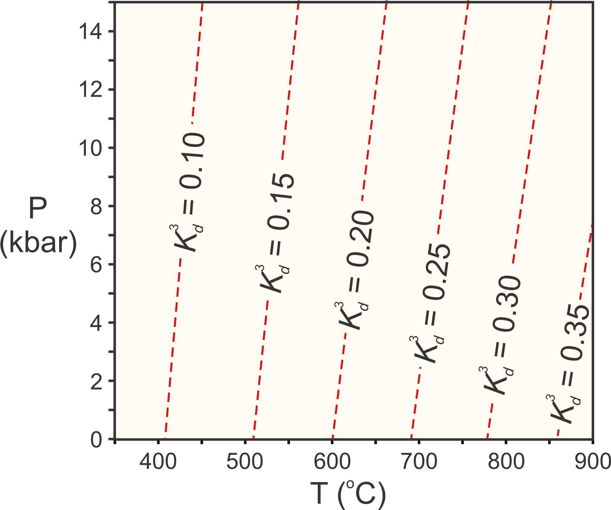
So, we can calculate diagrams such as the one in Figure 12.5 for exchange reactions. Figure 12.6 is such a diagram for the exchange of Fe and Mg between garnet and biotite (Reaction 6). In this diagram, the red lines are for values of K³_d, because cubing K_d keeps the values between 0 and 0.5 for typical metamorphic conditions. We could, however, have calculated and plotted K_d instead. Figure 12.6 depicts what we call the garnet-biotite geothermometer.

 

12.4 Thermobarometry

Metamorphic petrologists are often concerned with determining the pressure and temperature at which a rock equilibrated. This process is thermobarometry. If we can learn the P-T conditions at which a rock equilibrated, we can make inferences about how and where the rock formed. For example, rocks from deep within Earth equilibrate at high pressures and high temperatures. In contrast, rocks metamorphosed in a subduction zone commonly equilibrate at high pressures but relatively low temperatures. Thus, thermobarometry can help us determine rock genesis and also interpret tectonic settings. Thermobarometry is often sometimes used to evaluate variations in metamorphic grade across a metamorphic terrane.

. . . the minerals present in a metamorphic rock, and the compositions of those minerals, record the conditions at which equilibrium occurred.

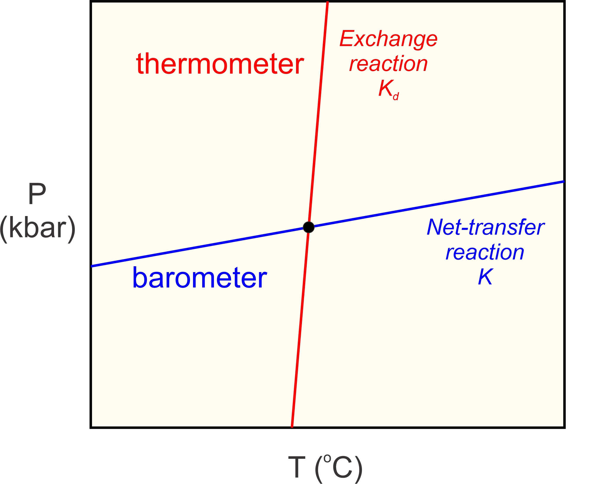
The underlying principle of thermobarometry is that the minerals present in a metamorphic rock, and the compositions of those minerals, record the conditions at which equilibrium occurred. The best metamorphic thermometers are based on mineral assemblages that form by reactions sensitive to temperature but not (much) to pressure (red line in Figure 12.7). The best metamorphic barometers are based on assemblages that are sensitive to pressure but not (much) to temperatures (blue line in Figure 12.7). Many rocks, unfortunately, do not contain assemblages that make suitable thermometers or barometers. Even when requisite assemblages are present, applying metamorphic thermometers or barometers requires knowing the compositions of the minerals in the rocks, information that may not be available. Nonetheless, thermobarometry has been widely applied to metamorphic rocks with great success.

Many commonly used thermometers are based on exchange reactions. Exchange reactions involve no change in mineralogy, and thus no significant change in volume. So, they are temperature-sensitive, but not very pressure-sensitive. They have steep slopes on P-T diagrams (Figure 12.7). The most common exchange thermometers involve Fe²⁺ and Mg distributed between two minerals such as garnet and biotite (Reaction 6), or garnet and clinopyroxene. Other exchange reactions, involving different elements, also may record temperature – for example the exchange of Fe²⁺ and Ti between titanium-bearing magnetite and ilmenite.

Petrologists have calibrated many potential thermometers using experimental results, thermodynamic data, or both. For example, the composition of coexisting plagioclase and hornblende can be used to estimate temperature. Other thermometers involve trace element concentrations of phases. For example, the concentrations of Ti in quartz (SiO₂) and zircon (ZrSiO₄) in equilibrium with rutile (TiO₂), and the concentration of Zr in rutile are very sensitive to temperature. We can apply these thermometers to igneous and metamorphic rocks, but it requires an ion microprobe for analysis of trace concentrations (ppm) of Ti and Zr. Another trace element thermometer with applications to metamorphic rocks involves the yttrium concentration of coexisting monazite and garnet (or monazite and xenotime).

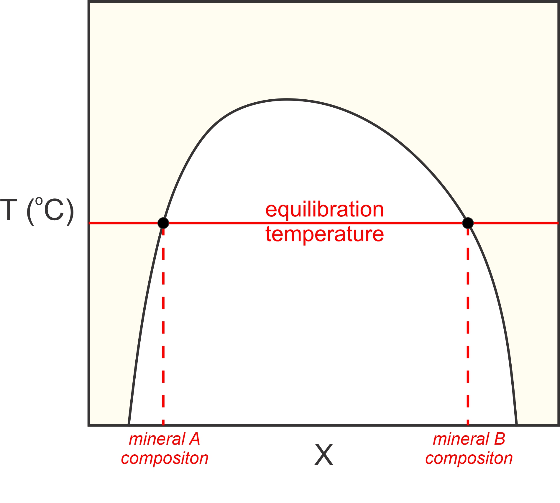
Petrologists also sometime use solvus thermometry to determine metamorphic temperatures. We looked at solvus relationships in igneous rocks earlier (in Chapter 8). There, we were considering minerals that were a homogeneous solid solution at high temperature but subsequently “unmixed” into two separate minerals during cooling. In contrast, metamorphic solvus thermometry involves two phases that most often obtained their compositions during heating (prograde metamorphism). Prograde or retrograde, the compositions of the coexisting minerals can tell us the temperature (Figure 12.8) at which the minerals equilibrated. For example, metamorphic petrologists use the solvus between calcite and dolomite, the solvus between plagioclase and alkali feldspars, and the solvus between orthopyroxene and clinopyroxene, as thermometers. We discussed these solvi in Chapter 8.

12.4.1 Thermometry

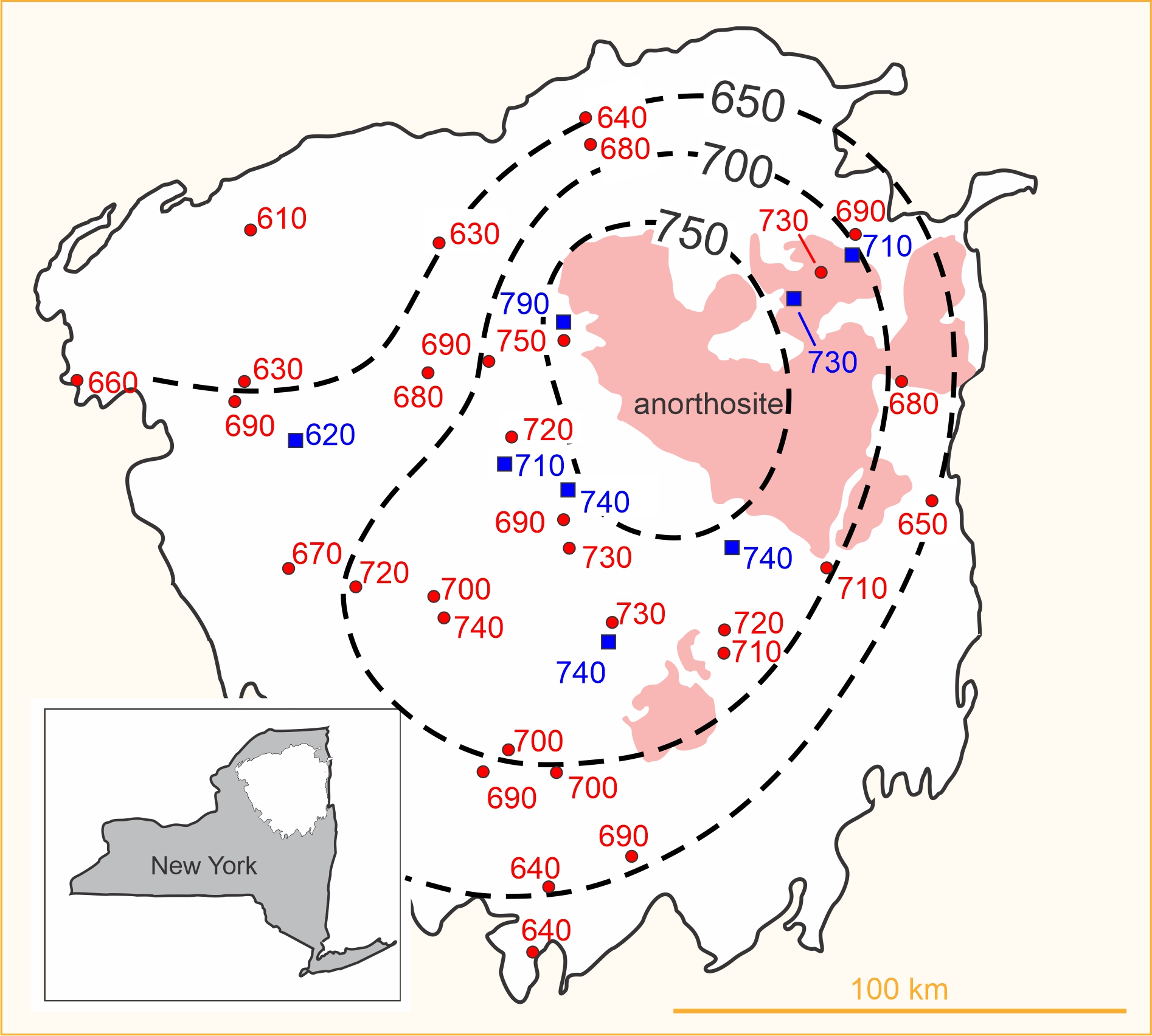
In one of the first large-scale applications of thermometry, Bohlen and Essene (1977) studied regional variations in metamorphic temperatures recorded by about 40 rocks from the Adirondack Mountains of New York. They used alkali-feldspar solvus thermometry and the magnetite-ilmenite Fe-Ti exchange thermometer. Each temperature plotted in Figure 12.9 was calculated using mineral compositions from different rocks. The temperatures in red are feldspar temperatures and the temperatures in blue are Fe-Ti oxide temperatures. The thermometry reveals that metamorphic temperature was greatest near the large plutonic anorthosite intrusion (shown in light red in the map) in the center of the mountains. For several reasons, Bohlen and Essene concluded that the temperatures recorded by the thermometers were peak metamorphic temperatures.

Besides mineral net-transfer and exchange reactions, metamorphic petrologists have also determined metamorphic temperatures using the concentration of stable isotopes, such as oxygen and carbon, in coexisting minerals. Isotopic variations record the temperature at which a system became closed to isotopic exchange. For example, the O¹⁸/O¹⁶ ratio in coexisting quartz and magnetite has been used as a thermometer, as has the C¹³/C¹² ratio in coexisting quartz and calcite, or calcite and graphite. In one study, Quinn et al. (2016) studied the isotopic composition of quartz inclusions in garnet from the Adirondacks. They found regional temperature variations nearly identical to those of Bohlen and Essene that are depicted in Figure 12.9.

12.4.2 Barometry

Traditional geobarometers involve net transfer reactions that have shallow slopes on P-T diagrams (Figure 12.7). The most pressure-sensitive reactions involve a significant volume change, so that the PV term in Equation 1 is much greater than the TS term. Reaction 5 is one example. Other barometers involving net transfer reactions include the reaction of pyroxene to fayalite and quartz, the Al₂O₃ content of pyroxene in equilibrium with garnet, and the reaction of garnet and quartz to pyroxene and feldspar.

Some barometers do not involve net-transfer reactions. They may involve the concentration of an element or component in a single mineral in equilibrium with a particular assemblage. For example, sphalerite (ZnS) in equilibrium with pyrite (FeS₂) and pyrrhotite (Fe_1-xS) always contains some FeS. The amount of FeS does not vary with temperature but does vary with pressure. So, sphalerite barometry has been applied to regionally metamorphosed rocks.

Metamorphic petrologists commonly combine thermometry and barometry to determine the unique pressure and temperature at which a rock equilibrated. Box 12.3 provides one example.

● Box 12.3 Example: Garnet-Biotite Thermometry and GASP Barometry The garnet-biotite thermometer and GASP barometer, discussed above in Section 12.3, have been widely applied to pelitic rocks. If a rock contains garnet, biotite, an Al2SiO5 mineral (kyanite, andalusite, or sillimanite), plagioclase, and quartz (a common assemblage) the thermometer and barometer together tell us the temperature and pressure of equilibration. A Garnet-Biotite Thermometer: Garnet and biotite are both solid solution minerals that contain Fe and Mg. Ferry and Spear (1978) conducted experiments and derived one of the original versions of the garnet-biotite thermometer. They found the following relationship between temperature (in Kelvin), pressure (in units of bars) and the distribution of Fe and Mg between the two minerals (expressed as Kd and calculated with Equation 14): [Eqn 15] TK = (2089 + 0.009562 P) / (lnKd + 0.7822) A GASP Barometer: Although the grossular component in pelitic garnets is generally quite low, if kyanite and quartz are present, grossular in garnet must be in equilibrium with anorthite in plagioclase or Reaction 5 will go to the right or left until equilibrium is obtained. [Rxn 5] grossular + 2 kyanite + quartz = 3 anorthite Ca3Al2Si3O12 + 2 Al2SiO5 + SiO2 = 3 CaAl2Si2O8 Hodges and Crowley (1985) calibrated Reaction 5 as a geobarometer. According to their calibration, the equilibrium constant for Reaction 5 is: [Eqn 16] KGr-An =(1.03XGt Ca / 1.35 XPl An)3  Then, the equilibration pressure may be calculated: [Eqn 17] Pbars = 1.258 TK (lnKGr-An + 18.474) – 8453 (The above expression is slightly different if a rock contains sillimanite instead of kyanite.) Example: Suppose we have obtained a chemical analysis for garnet and biotite that coexist with kyanite and quartz in Rock 1, a metapelite. Assume the analyses tell us that: 123(Fe/Mg) in garnet = 6.050 123(Fe/Mg) in biotite = 1.525 123XCa in anorthite = 0.186 Thus:      Kd = 3.967 according to Equation 14      KGr-An = 0.00084 according to Equation 16 We can use the values for Kd and KGr-An, along with Equations 14 and 16, to calculate the temperature and pressure at which Rock 1 equilibrated. The temperature calculated with Equation 14 depends, to a small extent, on a chosen pressure. And, the pressure calculated with Equation 16 depends on a chosen temperature. So we use an iterative approach to solve the two equations simultaneously: • We assume a pressure, and use Equation 15 to estimate the equilibration temperature. • Then we use that temperature and Equation 17, to derive the equilibration pressure. • We then use this new pressure to calculate a new temperature. • And we use the new pressure to calculate a new pressure, and so forth. • And after three or four iterations, the values will no longer change. When we do this, using the compositions of garnet and anorthite in Rock 1, we find that it equilibrated at 716 oC (989 K) and 6,360 atmospheres pressure. Try it for yourself!

12.4.3 Uncertainties

We can calculate statistical uncertainties in thermobarometric calculations by propagating errors from all stages of the P-T determinations: the mineral composition analyses, the thermodynamic data, and the calibration method. Typical uncertainties are ± 50°C, ± 1 kbar. However, there are other complications due to assumptions made.

Common sources of error in thermobarometric calculations include: 
• The assumption that the minerals record equilibrium conditions may not always be valid.
• The choice of mineral compositions to use in thermobarometric calculations is easy if all phases are homogeneous, but if minerals are compositionally zoned, the selection of compositions to use can be more uncertain.
• The stability of minerals may be affected by the presence of components that are difficult to analyze with standard techniques. For example, electron microprobe analyses do not distinguish between Fe²⁺ and Fe³⁺, but the difference is important. A thermobarometric calculation may be substantially in error if all Fe is assumed to be Fe²⁺ for minerals that contain substantial Fe³⁺.
• Thermobarometric calculations rely on thermodynamic data and a “calibration” that allows mineral composition to be related to temperature or pressure. The mineral compositions of the rock we are studying, therefore, should not be too different from the compositions on which the calibrations are based.
• Temperature calculations require an estimation of pressure, and pressure calculations require an estimation of temperature.

12.4.4 What Do Calculated P-T Conditions Mean?

For igneous rocks, thermobarometric results likely represent the conditions at time of crystallization, particularly for rapidly cooled rocks. Metamorphic rocks have more complex thermal and pressure histories, as we discussed in Chapter 9. The most common interpretation of thermobarometry is that minerals record the pressure and temperature conditions at the thermal maximum (peak of metamorphism) (Figure 9.32). The thermal maximum, however, may not represent the pressure maximum.

Additional complications arise because petrologists have established that some metamorphic rocks undergo retrogression during cooling. We can sometimes see evidence for retrogression of net transfer reactions by looking at rocks in thin section. By examining textures and mineral relationships, we can often determine if the mineral assemblages/textures are consistent with the notion that mineral compositions have preserved peak-metamorphic conditions that have not been overprinted during later events. Retrogression of exchange reactions is more difficult to see or measure. Multiple studies have demonstrated that Fe and Mg, for example, sometimes redistribute during cooling after the peak of metamorphism. It is likely that other elements do too. Nonetheless, for most rocks, most of the time, thermobarometry provides a good estimate of the conditions at which the rocks formed.

 

● Figure Credits Almost all graphics/photos in this chapter came from the authors and other primary contributors to this book. Figure 12.9 was based on a figure from Bohlen and Essene (1977).