11 Metamorphic Equilibria
KEY CONCEPTS
- The Laws of Thermodynamics govern mineral stability.
- Minerals and mineral assemblages in rocks may be stable, unstable, or metastable.
- Phase diagrams show conditions (stability fields) where different minerals or assemblages are stable.
- Reaction lines on phase diagrams show discontinuous reactions that separate stability fields.
- Reaction lines may intersect at invariant points where one or more reaction may become metastable.
- Continuous reactions do not plot as lines on phase diagrams but occur over a range of conditions.
- Net-transfer reactions involve a mineral or assemblage being replace by another; exchange reactions involve the exchange elements between minerals with no change in mineral abundance.
- Net transfer reactions may be solid-solid reactions, dehydration reactions, decarbonation reactions,
carbonation reactions, hydration reactions, or mixed volatile reactions. - The number of phases that can be stable together depends on the number of components of a chemical system. More components means more phases.
- The number of phases that can take place in a reaction depends on the number of components of a chemical system. More components means more phases.
- We can plot mineral compositions on binary and triangular composition diagrams.
- If we have more than three components we must use projections to plot mineral compositions on composition diagrams.
- The most commonly used kinds of projections are ACF diagrams, AFM diagrams, and Thompson AKFM projections.
- Petrogenetic grids are complex phase diagrams that show many reactions for model systems.
- Pseudosections show stability fields for different assemblages but only apply to a rock or a single composition.
11.1 Stable, Metastable and Unstable Equilibrium
Petrologists consider mineral reactions and construct phase diagrams to predict what will happen to a rock during metamorphism. We also use the same diagrams to interpret how a particular rock may have formed. The Laws of Thermodynamics govern phase equilibria and phase diagrams. In this chapter we will look at some important implications of those laws; we will discuss thermodynamics in more detail later in Chapter 12.
The Laws of Thermodynamics tell us that chemical systems, including minerals in rocks, are most stable when chemical energy is minimized. If a system has the minimum possible chemical energy, we say it is at stable equilibrium, or simply that it is stable. If a system is not at stable equilibrium, chemical reactions may occur until the system eventually reaches stability.
Metamorphic petrologists are often concerned about the conditions that make individual minerals or assemblages stable, because this knowledge allows interpretation of a rock’s history based on the minerals it contains. Quartz, feldspar, and a few other minerals are stable over a very wide range of metamorphic conditions. But most minerals and mineral assemblages are not, and they only occur in rocks that equilibrated within a specific range of pressure and temperature conditions. Thus, they have a restricted stability range.
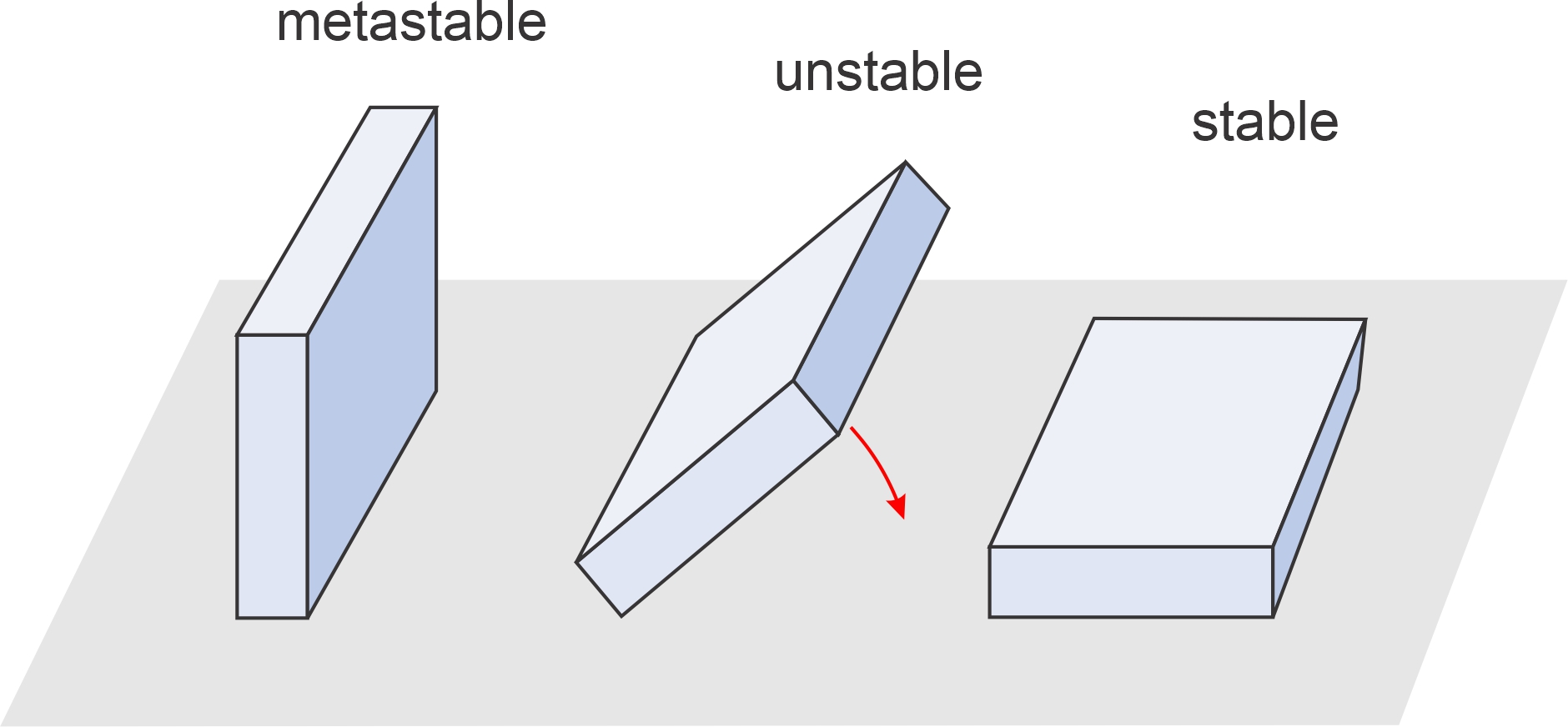
Figure 11.1 shows three rectangular slabs that are in metastable, unstable, and stable positions. The stable slab, lying on its largest side, has the least gravitational potential energy. The metastable slab, with somewhat greater potential energy, is temporarily in equilibrium, but could tip over if pushed. The unstable slab is teetering – on its way from being metastable to stable. Chemical systems behave like gravitational systems. They tend towards stable equilibrium – the conditions of lowest chemical potential energy – but may sometimes be metastable. For another simple comparison of stable, metastable, and unstable equilibrium conditions, follow this link to Chapter 8.
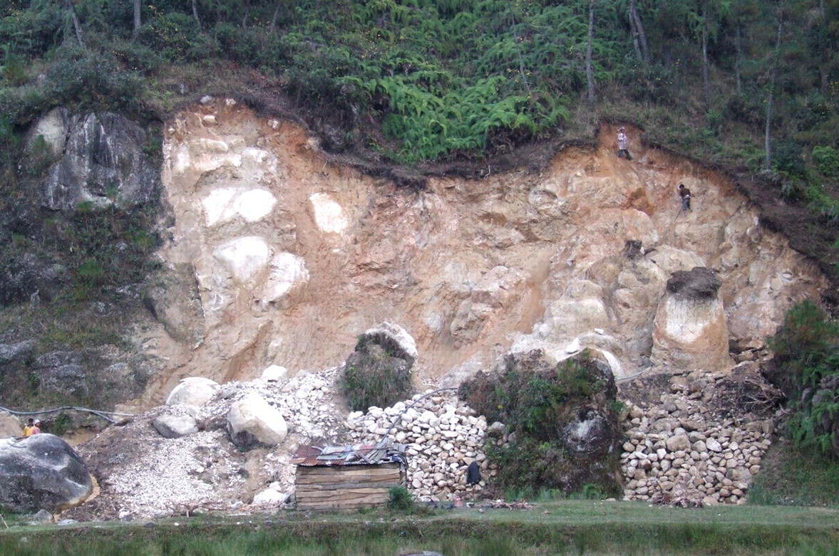
Unstable minerals are minerals undergoing reactions (perhaps very slowly) to produce more stable reaction products. For example, feldspars (unstable in outcrops at the surface) weather over time to become clay, which is stable. Weathering is an ongoing process that may occur quite slowly. For example, Figure 11.2 is a photo of (what was once) an outcrop of granite in India. Weathering, involving reaction of K-feldspar and quartz with water, has substantially replaced the granite with clay and Fe-oxides. The process has not, however, gone to completion, and the white colored pieces of rock are still solid granite. We call such remnants surrounded by highly weathered material, corestones. Given enough time, the corestones will completely break down and disappear.
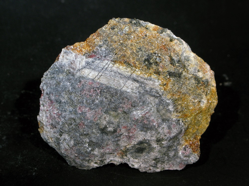
Weathering at Earth’s surface is commonplace, but often does not go to equilibrium. Thus we have, at Earth’s surface today, samples of minerals that are only stable at conditions deep within Earth. The term metastable refers to these minerals that should, in principle, be reacting to form more stable materials, but are not. For example, we find metastable sillimanite and garnet in outcrops of metamorphic rocks. Figure 11.3 is a sample collected in Rollins State Park, New Hampshire. Both garnet and sillimanite are unstable under normal Earth surface conditions and should, in principle break down into other minerals – but often they do not.
Diamond is, perhaps, the most classic example of a metastable mineral. Diamond consists of carbon, just like the common mineral graphite that makes up pencil lead. Diamond is only stable at pressures found at depths in Earth greater than 150 km or so. The Laws of Thermodynamics tell us that all the diamonds that we see should react to form graphite, yet we have many (metastable) diamonds to enjoy.
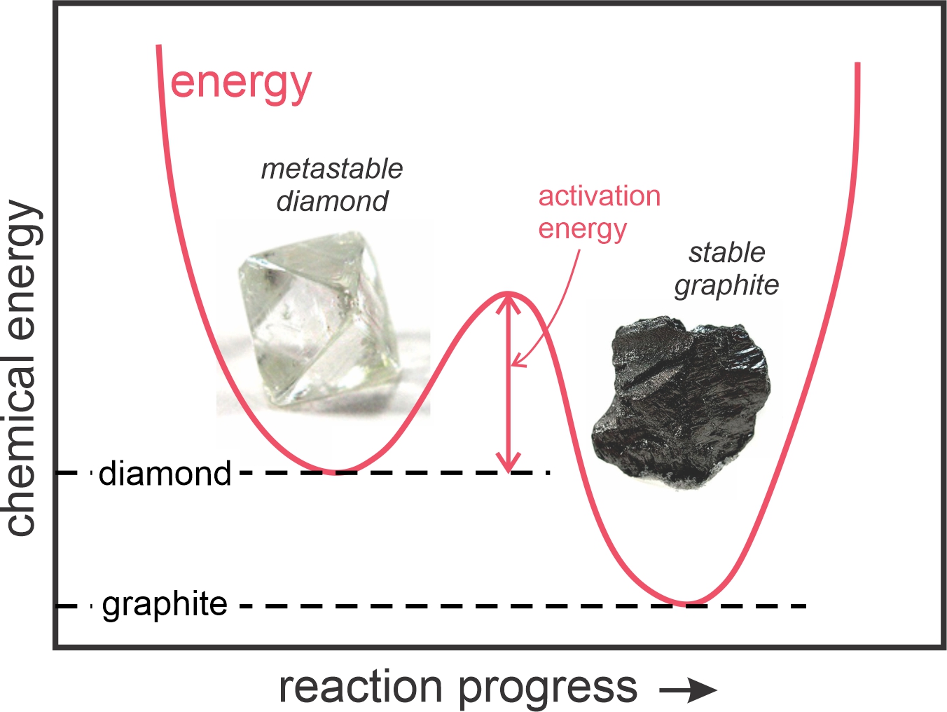
Disequilibrium and metastable minerals are common at Earth’s surface for two reasons: (1) some chemical reactions require a certain amount of activation energy to get started; and (2) at low temperatures, mineral reaction rates are slow – it may take a very long time for them to go to completion. Figure 11.4 depicts the relative chemical energies of diamond and graphite at Earth’s surface. Diamond has greater energy, but there is an energy “hump,” a certain amount of activation energy that must be overcome for diamond to turn into graphite. Because of activation energy, diamond, garnet, and other metastable minerals abound at Earth’ surface. At high temperatures within Earth, however, activation energies generally do not pose a problem, and reaction rates are faster than at the surface. So, rock and mineral systems typically attain stable equilibrium.
11.2 Reaction Lines and Stability Fields on Phase Diagrams
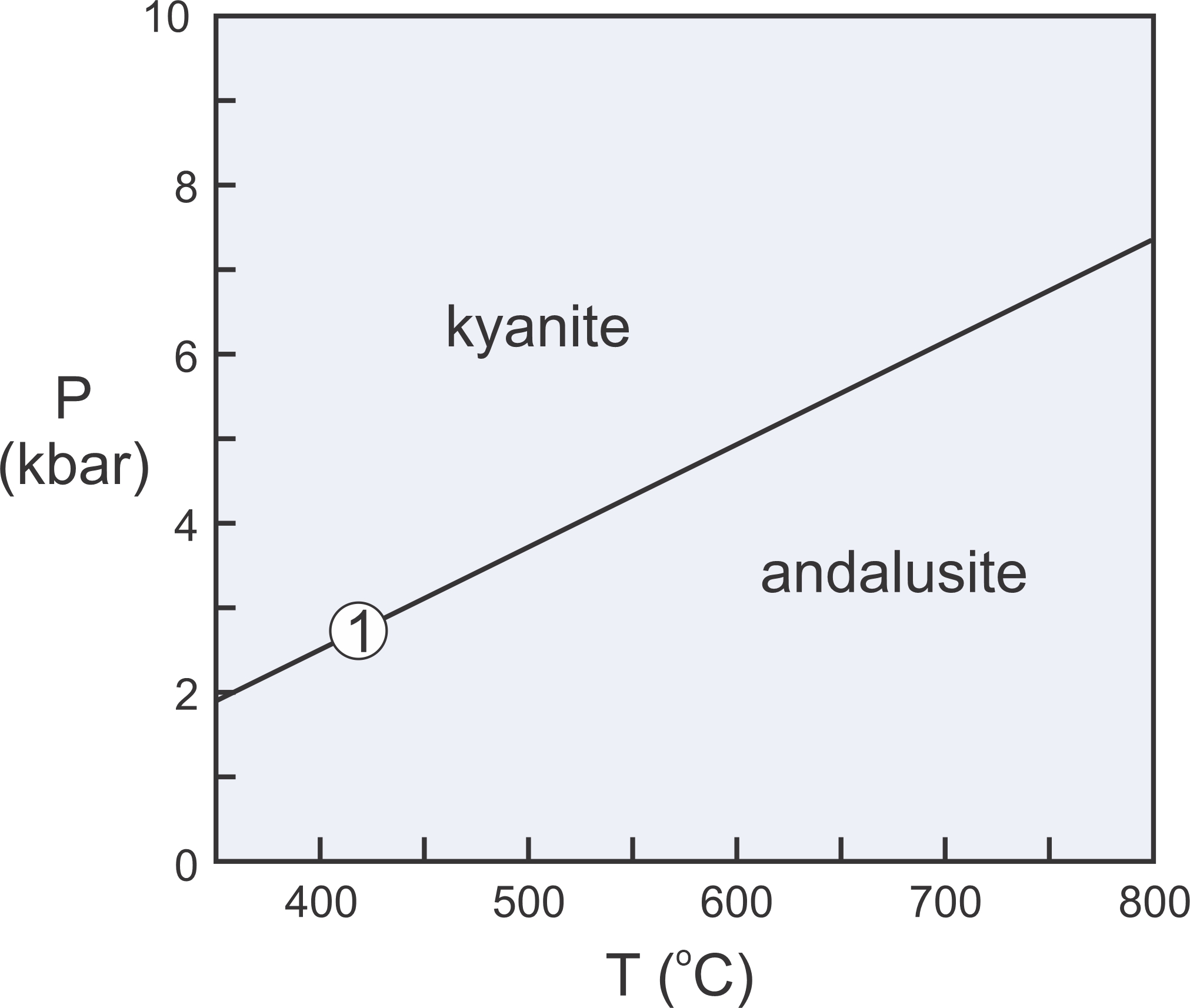
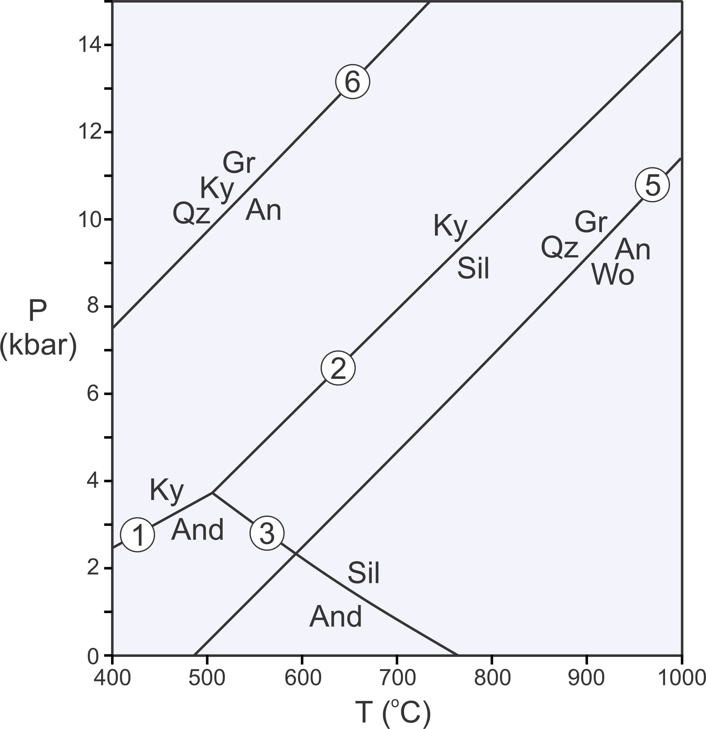
The Laws of Thermodynamics allow us to construct phase diagrams and to predict which minerals form under particular conditions. We use metamorphic phase diagrams like the one seen here in Figure 11.5 to show mineral equilibria that may affect stable minerals or mineral assemblages. This diagram has a reaction line that separates stability fields for kyanite and andalusite. We can write the reaction that occurs along this line as:
| [Rxn 1] | kyanite = andalusite Al2SiO5 = Al2SiO5 |
Kyanite and andalusite have the same composition, Al2SiO5, so this phase diagram is for a 1-component system. The diagram tells us that, in general, rocks that contain andalusite form at higher temperature than rocks that contain kyanite. By convention, we always put the high-temperature mineral or assemblage to the right of the equal sign when writing a reaction.
Kyanite is a high-pressure mineral, and andalusite is a low-pressure mineral. For a rock with composition Al2SiO5, we will get kyanite if P-T conditions are above the reaction line. We will get andalusite if conditions fall below the line. If conditions fall exactly on the line (unlikely), we may have both kyanite and andalusite stable together. So, most rocks will contain one or the other of the minerals, not both.
As discussed in Chapter 8, at high pressure, minerals of greatest density are most stable. At low pressure, minerals of lower density are stable. Additionally, minerals of greatest entropy are stable at high temperature. Minerals of lower entropy are stable at lower temperature. Thus, the phase diagram in Figure 11.5 tells us that kyanite is denser than andalusite, and kyanite has lower entropy than andalusite.
● Box 11.1 Reminder: Phases and ComponentsIn this chapter, we will be talking about phases and components in some detail. It is worthwhile reviewing the definitions of these terms before we go on. The term phase refers to any compositionally and physically distinctive substance. Phases must be homogeneous and can be solids, liquids or gases. Thus, minerals are phases. But, so too are magmas and other liquids, and gases. Rocks are not phases but are mixtures of phases, generally mostly minerals. Thermodynamics deals with chemical systems, and a chemical system is defined by its composition. That is, a chemical system is defined by the chemical components that make up everything in the system. We choose components for convenience. Generally we choose oxides such as CaO, Al2O3, or H2O, but we may choose individual elements are complex compounds when convenient and appropriate.
For an example of phases and components, we can consider a system containing the components Al2O3 and H2O. This system includes five common phases, three minerals, and H2O liquid and vapor. Each of these phases is made of some combination of Al2O3 and H2O. Diaspore and gibbsite, sometimes with boehmite (a polymorph of diaspore) are important aluminum ore minerals in bauxite deposits, a major source of aluminum today. These deposits form by weathering and leaching of aluminous parent rocks. Geological systems almost always contain more than two components, and may contain many different minerals or other phases. Different phases and phase assemblages are stable under different conditions. When conditions change, and a phase or assemblage of one sort changes into another, a phase change has occurred. |
||||||
11.2.1 A Simple Phase Diagram for Al2SiO5
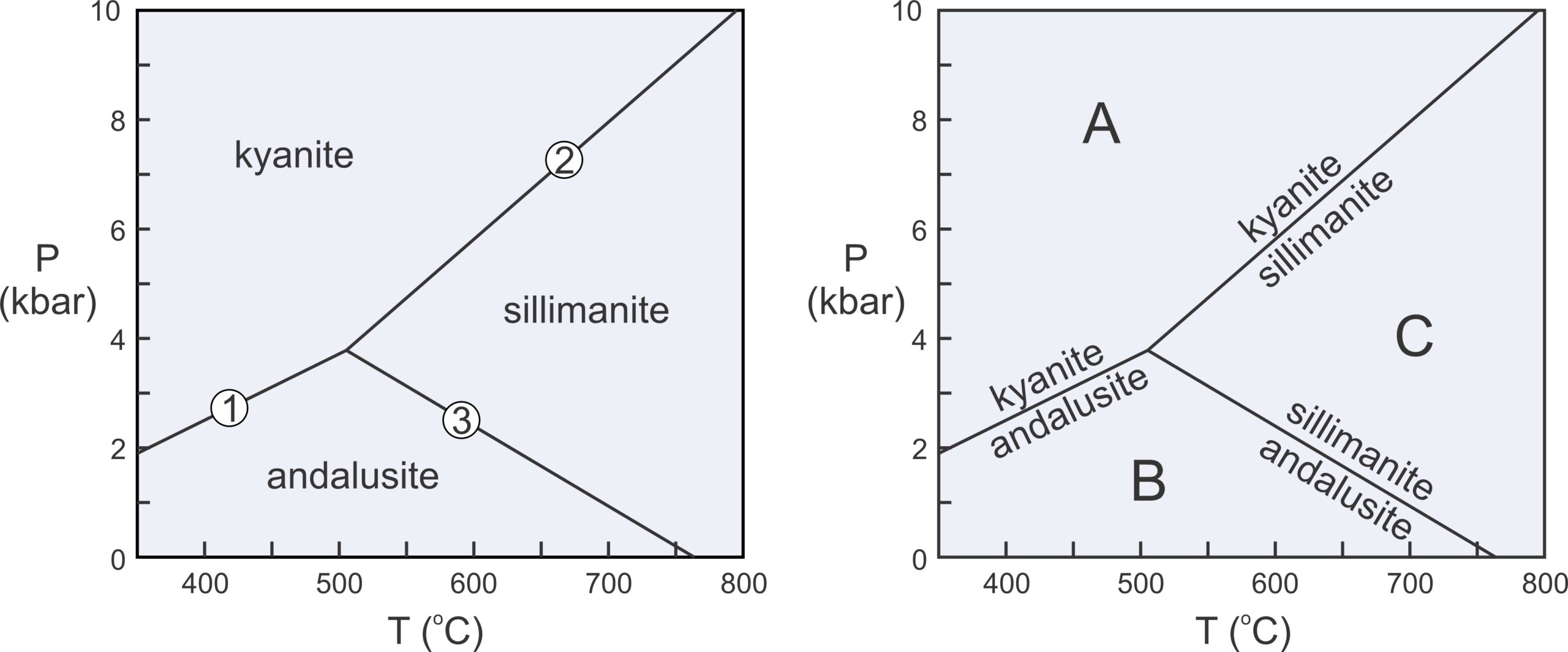
We considered kyanite and andalusite above, but besides these two minerals, the Al2SiO5 system contains a third polymorph, sillimanite. Figure 11.6 includes the phase relations involving all three of these minerals. The diagram on the left depicts stability fields for the three Al2SiO5 minerals. The different fields are the ranges of pressure and temperature where each polymorph is stable. Reaction lines separating the fields depict the conditions at which chemical reactions occur. Sillimanite will eventually form from either kyanite or andalusite if metamorphic temperature increases, and kyanite will eventually form from andalusite or sillimanite if pressure increases.
The two diagrams in Figure 11.6 depict the same things. The diagram on the right has reactions labeled instead of stability fields. Petrologists use both kinds of diagrams and they tell us the same things. Rocks containing kyanite form at relatively low temperature and high pressure (field A), rocks containing andalusite form at low pressure (field B), and rocks containing sillimanite form at relatively high temperature (field C). The diagrams also allow us to make predictions. For example, if a rock containing andalusite is metamorphosed at high temperature, the andalusite will change into sillimanite.
Phase diagrams for simple chemical systems may only contain a few reactions and may involve only a few components. The aluminosilicate diagram in Figure 11.6 is an example. All the minerals considered have the same composition. They contain a single component, Al2SiO5 and are related by three reactions:
| [Rxn 1] | kyanite = andalusite Al2SiO5 = Al2SiO5 |
| [Rxn 2] | kyanite = sillimanite Al2SiO5 = Al2SiO5 |
| [Rxn 3] | andalusite = sillimanite Al2SiO5 = Al2SiO5 |
These three reactions intersect at an invariant point, a point at a unique pressure and temperature (about 4 kbar and 500oC). If P-T conditions fall exactly on that point, all three Al2SiO5 polymorphs can exist stably together. If conditions fall on a reaction line, two polymorphs may coexist in equilibrium. If conditions are neither at the invariant point nor on a reaction line, a single polymorph will be stable.
11.2.2 Reaction Progress and Interpreting Phase Diagrams
Figure 11.7 is a phase diagram with a reaction (shown by the line and labels in black) that involves three minerals (pyrophyllite, diaspore, kyanite) and H2O:
| [Rxn 4] | pyrophyllite + 6 diaspore = 4 kyanite + 4 H2O Al2Si4O10(OH)2 + 6 AlO(OH) = 4 Al2SiO5 + 4 H2O |

It is worth emphasizing that Reaction 4 limits the conditions where pyrophyllite and diaspore can coexist (lower temperatures). It also limits where kyanite and H2O can coexist (higher temperatures). But it does not limit where any of the four phases are stable by themselves. Kyanite, for instance, is stable to the left of the Reaction 4 (in Figure 11.7) as long as water is not present. This is an important point because many people look at a diagram like this and interpret it to mean that kyanite can only exist at high temperature (because Ky appears on the right side of the reaction). The diagram, instead, tells us that kyanite with H2O can only exist at high temperature – a big difference.
Suppose a rock at low temperature contains mostly kyanite and pyrophyllite with a small amount of diaspore. If heated, conditions will eventually reach the reaction curve, and pyrophyllite and diaspore will react to produce kyanite and H2O (as shown by the red arrows and labels Figure 11.7). The reaction will progress, and temperature will not increase until it goes to completion. Because the parent rock in this example contained only minor diaspore, only a small amount of reaction will occur before the diaspore is gone. If temperature increases further, kyanite and H2O produced by the reaction will join leftover kyanite and pyrophyllite, and the rock will contain kyanite, pyrophyllite, and H2O. This is true for a protolith that contains lots of kyanite and pyrophyllite and only a small amount of diaspore. It is not necessarily true for rocks of other compositions.
One key point that often leads to confusion, is that phase diagrams do not tell us which minerals or mineral assemblages will be present in a rock. There are generally many possibilities and the stable mineral or assemblage, as pointed out in the previous paragraph, depends on rock composition. Instead, phase diagrams tell us which minerals or mineral assemblages are unstable (will not be present) under different conditions. To clarify this, let’s consider Reaction 4 again.
Consider a rock made of some mix of pyrophyllite, diaspore, kyanite, and H2O. The rock may contain one, two, three, or all four of these phases. There are 15 possible combinations in all. Assuming the rock is at equilibrium, the stable mineral assemblage varies predictably with rock composition and P-T conditions. Figure 11.8 shows where each of the 15 assemblages is stable.

Although Reaction 4 relates the four phases, by itself each of the four is stable on both sides of the reaction. Some phase pairs, too, are stable everywhere. Other pairs, however, have restricted stabilities. Pyrophyllite and diaspore (with or without a third phase) are only stable together to the left of the reaction line. Kyanite and H2O (with or without a third phase) are only stable together to the right of the reaction line. Thus, three of the possible assemblages (in red in Figure 11.8) are stable to the left of the curve. Three other assemblages (in blue) are stable to the right. The single 4-phase assemblage (Py-Dsp-Ky-H2O) is only stable for P-T conditions that plot exactly on the reaction line. The other eight possible assemblages are stable everywhere and are not affected by the reaction, So, individual reactions on phase diagrams only affect rocks of particular compositions and may not affect some rocks or mineral assemblages at all.
11.3 More Complicated Reactions
Reactions 1 – 3, above are simple reactions involving only two minerals. Reaction 4 involves four phases (3 minerals and H2O). Metamorphic reactions, however, can be much more complicated, sometimes involving five or more phases. And, reactions can be of many kinds. Some involve only solid minerals, like Reactions 1, 2 and 3. Others may involve H2O or CO2 or other vapor phases, like Reaction 4.
11.3.1 Solid-Solid Reactions
Reactions 1, 2, and 3 are solid-solid reactions. This means they do not involve H2O, CO2, or other vapor phases. Solid-solid reactions generally plot as straight, or near-straight, lines on P-T diagrams. Reactions 5 and 6 (below) are two more examples of solid-solid reactions:
| [Rxn 5] | grossular + quartz = anorthite + 2 wollastonite Ca3Al2Si3O12 + SiO2 = CaAl2Si2O8 + 2 CaSiO3 |
| [Rxn 6] | 3 anorthite = grossular + 2 kyanite + quartz 3 CaAl2Si2O8 = Ca3Al2Si3O12 + 2 Al2SiO5 + SiO2 |
The phase diagram in Figure 11.9 contains all five solid-solid reactions that we have considered (Reactions 1, 2, 3, 5, and 6). Unlike Reactions 1, 2, and 3, however, Reactions 5 and 6 involve four phases. As written above, these reactions are balanced – they contain reaction coefficients that are not all equal to 1. Often, especially when we label reactions on phase diagrams, we omit the reaction coefficients for simplicity and to save space, as has been done in Figure 11.9 – and in most other figures in this chapter. Additionally, also to save space, we normally use mineral abbreviations on phase diagrams as is done for most of the diagrams in this chapter. The abbreviations are defined in Box 11.2.
● Box 11.2 Minerals, Abbreviations and FormulasThe table below lists minerals, their abbreviations (used primarily in figures), and mineral formulas. For the rest of this chapter, we will omit mineral formulas from reactions and just use mineral names.
|
|||||||||||||||||||||
11.3.2 Dehydration Reactions
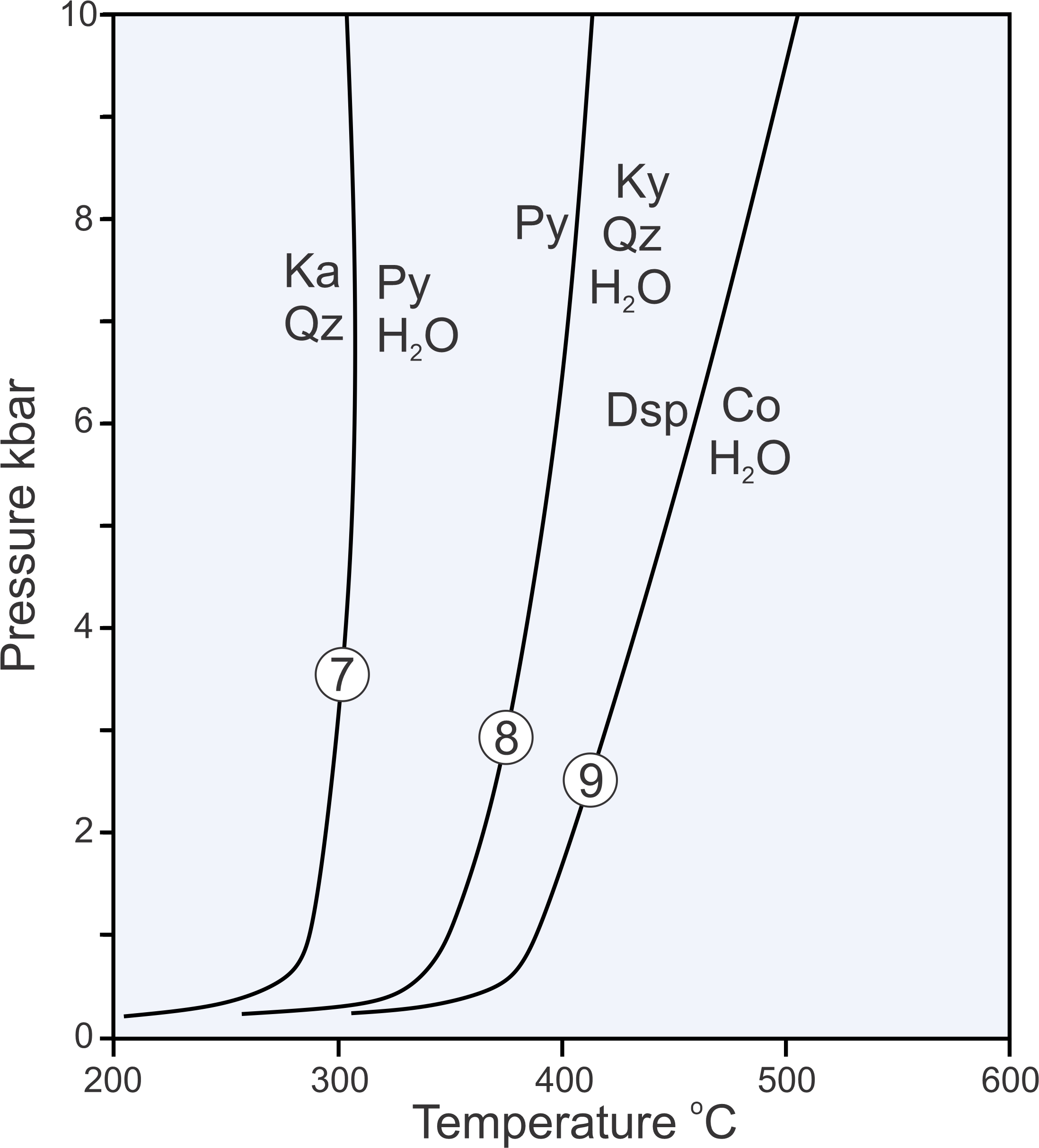
Reactions 7, 8, and 9, plotted on the phase diagram above in Figure 11.10, are examples of dehydration reactions:
| [Rxn 7] | kaolinite + 2 quartz = pyrophyllite + H2O |
| [Rxn 8] | pyrophyllite = kyanite + 3 quartz + H2O |
| [Rxn 9] | 2 diaspore = corundum + H2O |
When dehydration reactions occur, minerals that contain H2O (hydrous minerals) decompose to other (generally all anhydrous) minerals, releasing H2O. In contrast with most solid-solid reactions, dehydration reactions are not straight lines on phase diagrams. The curvature arises because the properties of H2O are not linear with pressure and temperature. Furthermore, the curves for dehydration reactions can never reach zero atmospheres pressure because, in an absolute vacuum, a hydrous mineral will always decompose to release H2O. So, at low pressure, the reaction lines curve around and become tangential to the 0 pressure line. Although the lowest pressure in Figure 11.10 is 0, to avoid complications and to avoid clutter, we often do not run the pressure scale down to 0 when phase diagrams include dehydration reactions.
11.3.3 Decarbonation Reactions

Decarbonation reactions release CO2 when carbonate minerals react to make other minerals. For example, Reactions 10 and 11 (below) are common decarbonation reactions that occur during metamorphism of a limestone. These reactions are likely the origins of the wollastonite and diopside seen in Figure 11.11:
| [Rxn 10] | calcite + quartz = wollastonite + CO2 |
| [Rxn 11] | dolomite + 2 quartz = diopside + 2 CO2 |
Reactions 7 through 11 involve a single volatile phase (H2O or CO2). Some more complicated reactions, called mixed-volatile reactions, involve both H2O and CO2 – for example:
| [Rxn 12] | tremolite + 5 calcite + 2 quartz = 5 diopside + H2O + 5 CO2 |
Dehydration, decarbonation, and mixed-volatile reactions result in volatile components (H2O, CO2, or both) being given off by minerals. The reactions take place with heating – it is sort of like the volatiles are being boiled out of the minerals – because H2O and CO2 in vapor form have much greater entropy (and thus lower energy) than they do as components in minerals. So, at high temperature, H2O- and CO2-bearing minerals become unstable. Thus, they are generally absent from high-grade metamorphic rocks.
Decarbonation and mixed-volatile reactions plot on P-T phase diagrams in the same way the dehydration reactions plot. More often, however, we look at these kinds of reactions on T-X diagrams (introduced in Chapter 8). We will talk more about T-X diagrams and look at many examples later when we consider metamorphism of carbonate rocks.
11.3.4 Carbonation and Hydration Reactions
Sometimes high-temperature minerals react to produce low-temperature minerals by carbonation or hydration reactions, such as:
| [Rxn 13] | forsterite + 2 CO2 = 2 magnesite + quartz |
| [Rxn 14] | 2 forsterite + 3 H2O = brucite + serpentine |
| [Rxn 15] | 6 forsterite + talc + 9 H2O = 5 serpentine |
Carbonation and hydration reactions commonly occur when high-temperature igneous rocks alter after being exposed to the elements at Earth’s surface. The reactions also occur during low-grade metamorphism of previously unmetamorphosed rocks of many sorts. They are especially important when ocean floor basalts are altered to become serpentinites. And, they occur during retrograde metamorphism that affects originally higher-grade metamorphic rocks in many settings.
|
|
|

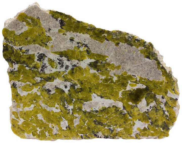
For example, hydration of plagioclase often produces saussurite (the green material in Figure 11.12). Saussurite is a mix of several minerals including, most significantly, epidote. And, hydration of mafic minerals can lead to the formation of H2O-bearing minerals including serpentine and brucite (perhaps by Reactions 14 and 15). The serpentinites seen previously in Figures 9.24 and 9.25 are products of hydration reactions. In these rocks, serpentine has replaced most of the original minerals. In other rocks, carbonation of olivine or other mafic minerals may lead to the formation of magnesite (for example, by Reaction 13). Figure 11.13 is a photo of magnesite-serpentine rock that formed by both carbonation and hydration of an ultramafic protolith. Reactions 13, 14, and 15 are only three of the many commonly occurring carbonation and hydration reactions.
11.3.5 Net Transfer and Exchange Reactions
The reactions we have considered so far in this chapter all involve a mineral or assemblage reacting to produce a different mineral or assemblage. We call such reactions net-transfer reactions. Net-transfer reactions involve chemical components being “transferred” from one phase or set of phases to others.
Exchange reactions, in contrast with net-transfer reactions, involve chemical components being “exchanged” between phases. Compositions change, but the minerals present do not. For example, consider a rock containing garnet and cordierite. Natural garnet contains several end-members, including Fe3Al2Si3O12 (almandine) and Mg3Al2Si3O12 (pyrope). Natural cordierite also contains Fe and Mg end members: Fe2Al4Si5O18 (Fe-cordierite) and Mg2Al4Si5O18 (Mg-cordierite). So we can write an exchange reaction:
| [Rxn 16] | 2 almandine + 3 Mg-cordierite = 2 pyrope + 3 Fe-cordierite |
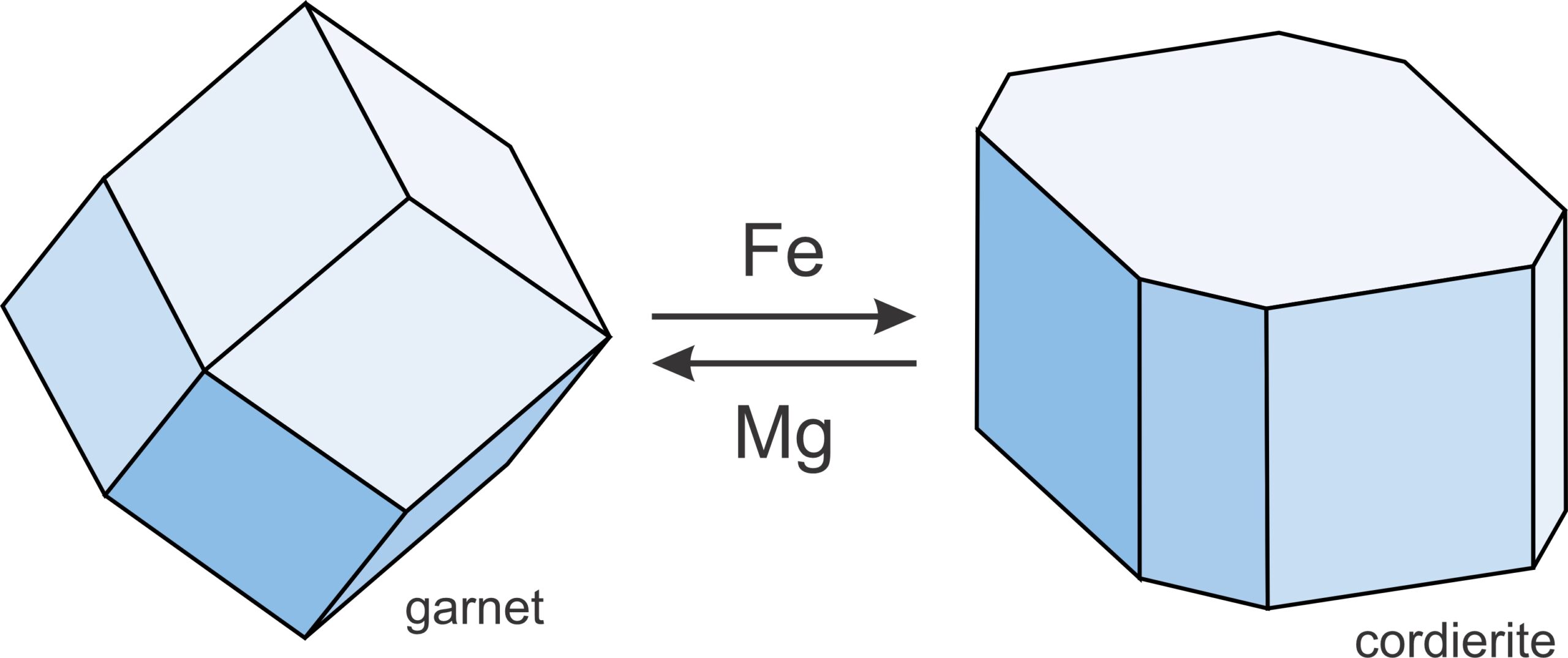
Garnet is always more Fe-rich than cordierite but, with increasing temperature, Reaction 33 proceeds to the right. Garnet becomes increasingly Mg-rich and cordierite becomes increasingly Fe-rich (Figure 11.14).
We can write similar reactions describing the exchange of Fe and Mg between any pair of mafic minerals, including garnet, cordierite, biotite, olivine, clinopyroxene, orthopyroxene and others. We can write reactions involving exchange of other elements too. No matter the elements involved, because exchange reactions have the same minerals on both sides of the equal sign, they involve little volume change and are much more sensitive to temperature variations than to pressure variations. This means we can sometimes use exchange reactions to estimate the temperature at which two minerals equilibrated. To make such estimates, however, requires that we know the actual chemical compositions of the (natural) minerals involved. Typically we get that information using an electron microprobe.
11.3.6 Discontinuous and Continuous Reactions
Most of the net-transfer reactions we considered previously are discontinuous reactions. This means they occur at a single temperature for any pressure and we can plot them as a line on a phase diagram. At temperatures below the line, one side of the reaction is stable. At temperatures above the line, the other side is stable. There is a discontinuity along the line. In contrast, exchange reactions are continuous reactions. Continuous reactions involve reactants and products that coexist over a range of pressure-temperature conditions, and involve changes in phase compositions when pressure or temperature change. Continuous reactions are more common than discontinuous reactions, and just about all metamorphic minerals change composition in response to changes in metamorphic grade.
In systems with multiple components and solid-solution minerals, most net transfer reactions are continuous. For example garnet, in the presence of sillimanite and quartz, may react upon heating to form cordierite by the following reaction:
| [Rxn 17] | 2 garnet + 4 sillimanite + 5 quartz = 3 cordierite |
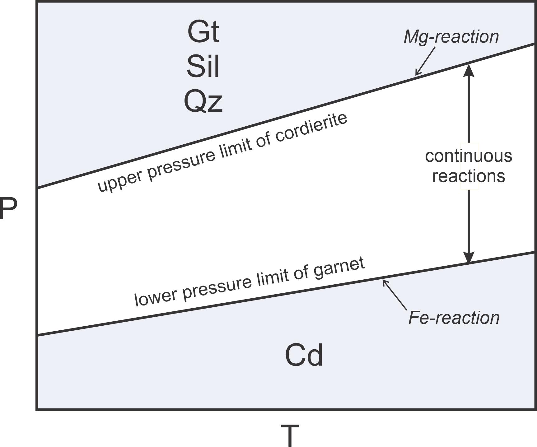
As pointed out above, garnet and cordierite, are solid solution minerals containing variable amounts of their Fe and Mg end members. Reaction 17 occurs at relatively low pressure if Fe-content is high, at elevated pressure if Mg-content is high, and somewhere between for intermediate compositions. So Reaction 17 is continuous and occurs over a range of conditions. Figure 11.15 shows these relationships schematically. At low pressure we get cordierite, at high pressure we get garnet, sillimanite, and quartz. And, at pressures between we may have all four minerals.
We call reactions, like Reaction 17, sliding reactions, because they slide up and down depending on mineral composition. In the space between the Fe- and Mg-reaction, both the exchange reaction (Rxn 16) and the net transfer reaction (Rxn 17) occur continuously as mineral compositions change with both pressure and temperature.
11.4 The Phase Rule
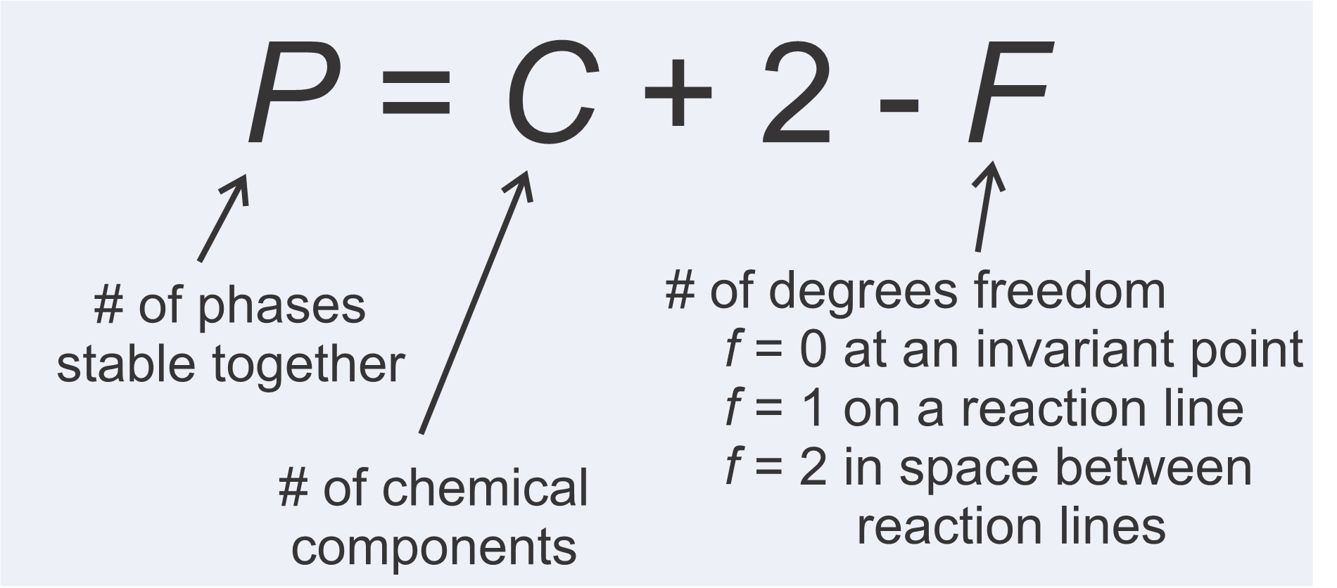
We just looked at some example reactions. Some contained two minerals and some contained more. Why is this? The answer is that the number of phases in a reaction depends on the number of chemical components involved. More components means reactions contain more phases. We also saw, in the examples above, that the largest number of phases are stable together if P-T conditions fall on an invariant points. One fewer are stable together on reaction lines, and the fewest number of phases are stable in fields between reaction lines. These observations are manifestations of the phase rule, depicted in Figure 11.16, promulgated by Yale professor J.W. Gibbs around 1875.
Interpreting the phase rule is straightforward. The number of phases that may coexist stably (P) is equal to the number of chemical components (C) plus 2, minus the number of degrees of freedom (F). F = 0 at an invariant point, because neither P nor T can change without leaving the point. F = 1 on a reaction line, because P and T can vary, but must vary proportionally to stay on the line. F = 2 in space between reaction lines because P and T can vary independently in open space. The phase rule tells us that more phases may coexist if P and T fall on an invariant point than if they fall on a reaction line, and more phases may coexist at conditions on a reaction line than in open areas on phase diagrams. Table 11.3 summarizes these relationships for systems of 1, 2, 3, or 4 components.
| Table 11.3 The Phase Rule | |||
| # of components (C) | # of phases in space between reactions (F=2) | # of phases involved in a reaction (F=1) | # of phases that may coexist at an invariant point (F=0) |
| 1 2 3 4 |
1 2 3 4 |
2 3 4 5 |
3 4 5 6 |
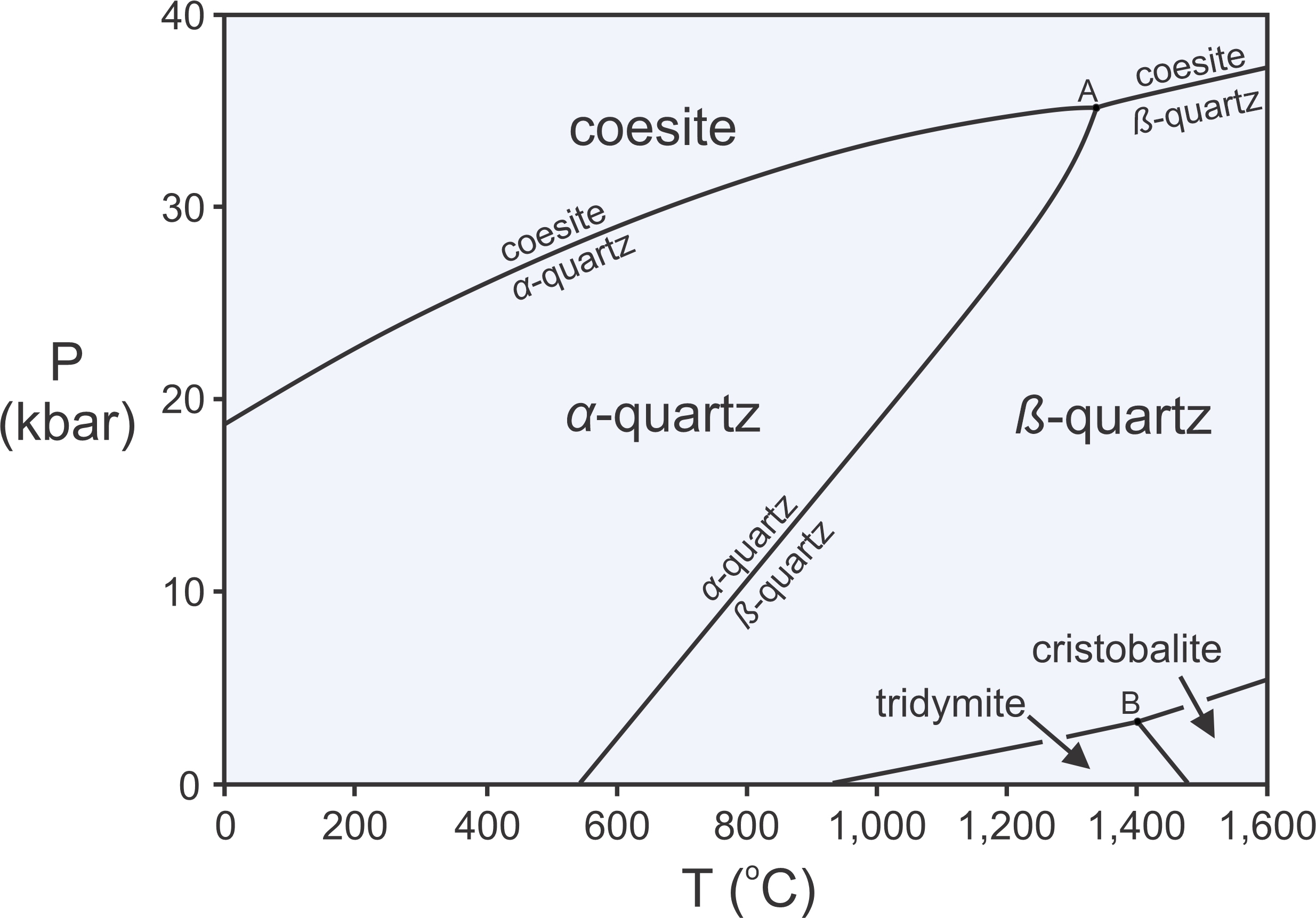
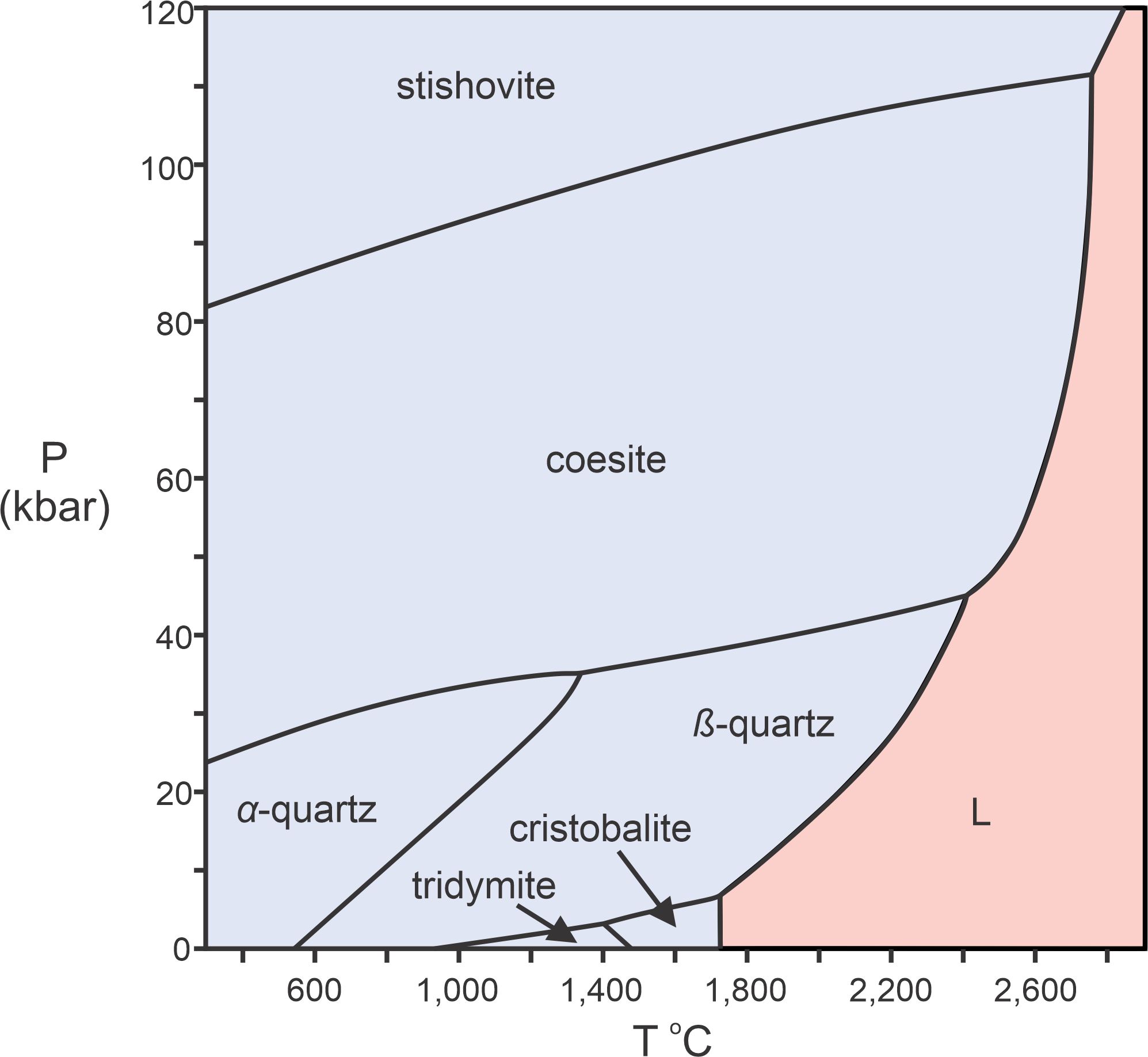
One important implication of the phase rule is that rocks that contain few components will contain relatively few minerals compared with rocks that contain more components. A quartzite, for example, may be made entirely of a single component, SiO2. Normally α-quartz will be present, as shown by the phase diagram in Figure 11.17. At elevated pressure or temperature, however, a rock may contain coesite , β-quartz, tridymite, or cristobalite instead of quartz. Still, under most conditions only one mineral will be present. In contrast with quartzites, metamorphosed shales contain half a dozen or more major components, and so may contain many minerals.
A second important implication of the phase rule stems from the observation that rocks are unlikely to equilibrate at conditions that fall on a reaction line. Furthermore, they are even more unlikely to equilibrate at conditions that fall on an invariant point, such as points A or B in Figure 11.17. Consequently, F = 2 most of the time, so the maximum number of phases that will coexist is equal to the number of components (most of the time). Petrologists sometimes call this observation the mineralogical phase rule.
11.4.1 1-Component Systems
Figure 11.17 is a phase diagram for the 1-component SiO2 system. We saw a larger and more complete diagram for this system in Chapter 8 (Figure 8.7). The SiO2 system contains half a dozen different polymorphs, all made of silica. According to the phase rule, reactions in 1-component systems always involve two phases. So reactions between the different polymorphs are simple, for example:
| [Rxn 18] | coesite = α-quartz |
The phase diagram in Figure 11.17 contains Reaction 18 and five others. Reaction lines lack labels in the lower-right part of the diagram, but the reactions can be inferred from the mineral names in adjacent fields. A single mineral (coesite, α-quartz, β-quartz, tridymite, or cristobalite) is stable in space between reaction curves. Two minerals may coexist along any reaction curve. Three minerals may coexist at either of the two invariant points where reaction curves intersect. Possible 3-mineral assemblages are coesite and α-quartz with β-quartz (point A), or tridymite and cristobalite with β-quartz (point B).
11.4.2 2-Component Systems
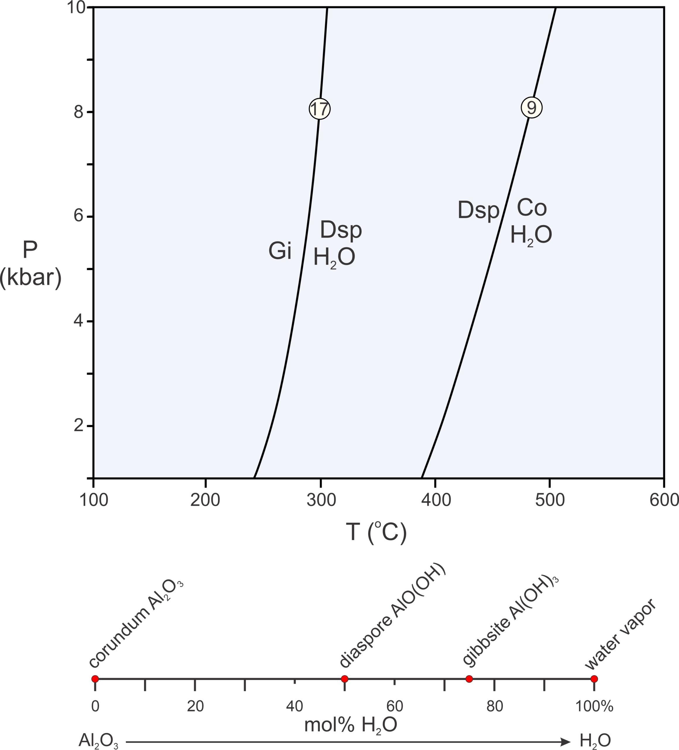
The P-T diagram in Figure 11.18 contains two example reactions in a 2-component system. The components are Al2O3 and H2O (see Box 11.1 for further discussion of this system), and each reaction involves three of four possible phases (3 minerals and H2O). The composition diagram below the phase diagram depicts phase compositions plotted on a line. We call diagrams that depict phase compositions, such as the one in the bottom of Figure 11.18, chemographic diagrams. In this example, the chemographic diagram is a line anchored by Al2O3 and H2O with red dots showing the different phase compositions.
As pointed out in Chapter 8, binary composition diagrams, like the one in the bottom of Figure 11.18, make it easy to identify possible chemical reactions. In 2-component systems, all reactions involve three phases, and they all involve one phase reacting to phases that plot on either side of it (or two phases reacting to produce one that plots between them) on a composition line. In this example, we are considering four minerals, so we can write four possible 3-mineral reactions (because each reaction is missing one of the four phases). The phase diagram in Figure 11.18 depicts two of them:
| [Rxn 19] | gibbsite = diaspore + H2O |
| [Rxn 9] | 2 diaspore = corundum + H2O |
Both reactions are dehydration reactions, and both curve on the P-T diagram in Figure 11.18. (Note that the pressure scale in this phase diagram does not go to 0 or the reaction curves would be significantly more curved and become tangential to the 0 pressure line.) A third reaction (not shown, off-scale to the left) tells us that gibbsite and corundum, if together, will always react to form diaspore. The fourth possible reaction (Rxn 20) is metastable, meaning that it cannot occur if a system is at equilibrium because the phases involved in the reactions will never be stable together:
| [Rxn 20] | 2 gibbsite = corundum + 3 H2O |
This reaction involves gibbsite and, so, could only occur to the left of Reaction 17 in Figure 11.18. But this reaction also involves corundum + H2O and so could only occur to the right of Reaction 9. Consequently, it can occur nowhere. The reason is that, with increasing temperature, gibbsite breaks down to diaspore before it can react to produce corundum.
As pointed out previously, phase diagrams do not tell us explicitly what minerals will be present under different conditions. There are many possibilities, and the stable mineral or assemblage depends on overall rock composition as well as on P-T conditions.
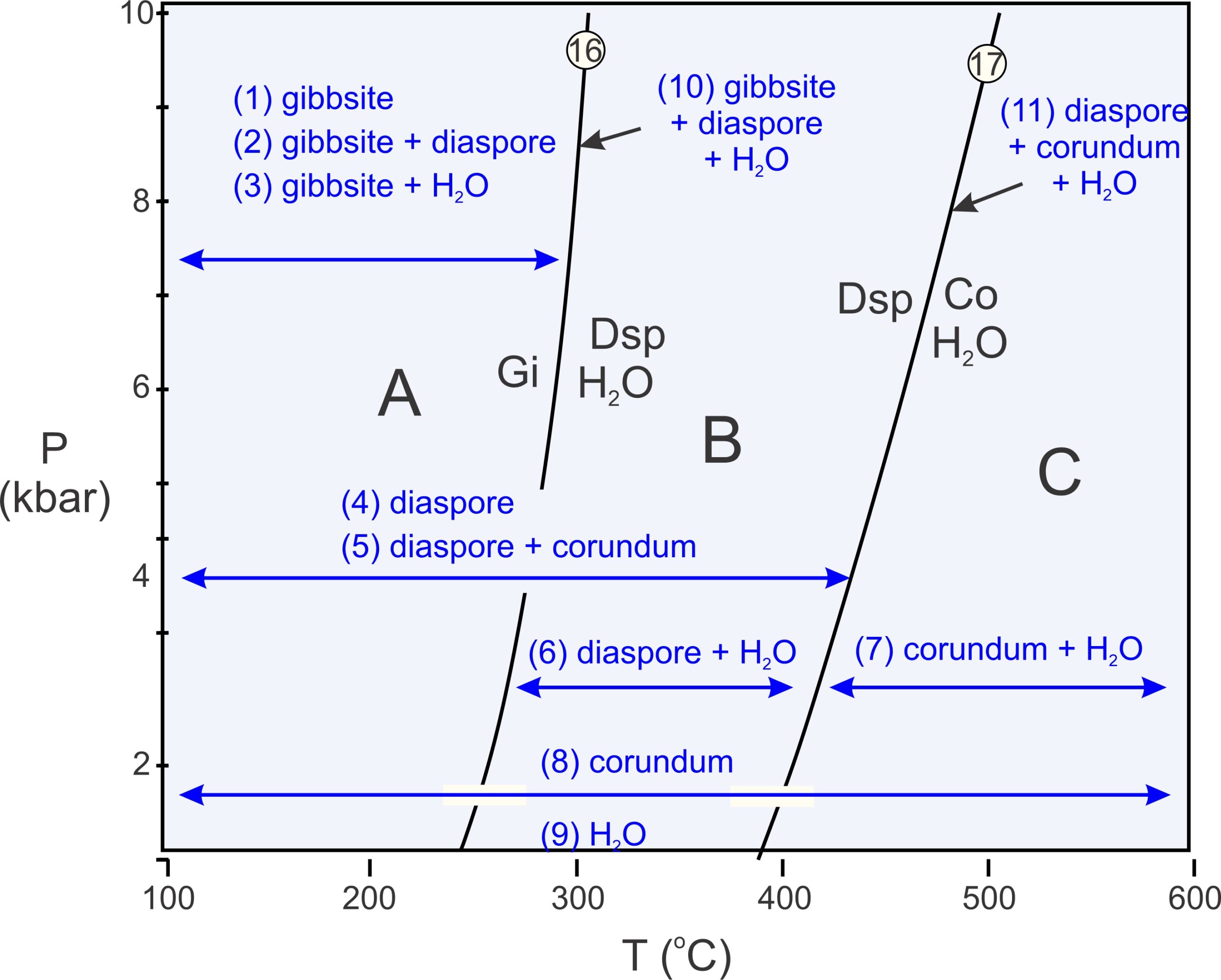
Figure 11.19 shows (in blue) the 11 possible assemblages for rocks with compositions equivalent to some combination of the Al2O3 and H2O. A rock may contain one mineral. If the mineral is gibbsite, the rock formed at conditions in field A, at low temperature. If the mineral is diaspore, the rock may have equilibrated in fields A or B. If the mineral is corundum it may have formed anywhere on the diagram. Stability fields for pairs of minerals (also shown and numbered in Figure 11.19) are more restricted. And, although unclear from this diagram, one mineral pair, gibbsite + corundum, is stable nowhere. Three minerals (assemblages 10 and 11) can only coexist along one of the two reaction lines. Four phases are never stable together.
11.4.3 3-Component Systems
Figure 11.20a, below, is a phase diagram for the 3-component Al2O3-SiO2-H2O system. To plot compositions in 3-component systems, we use triangular diagrams. The triangular diagram in Figure 11.20b depicts the compositions of the phases we are considering. The phase rule tells us that reactions in a 1-component system contain a maximum of two phases (e.g., Figure 11.17). Reactions in a 2-component system contain a maximum of three phases (e.g., Figure 11.18). And reactions in a 3-component system, like this one, contain a maximum of four phases.
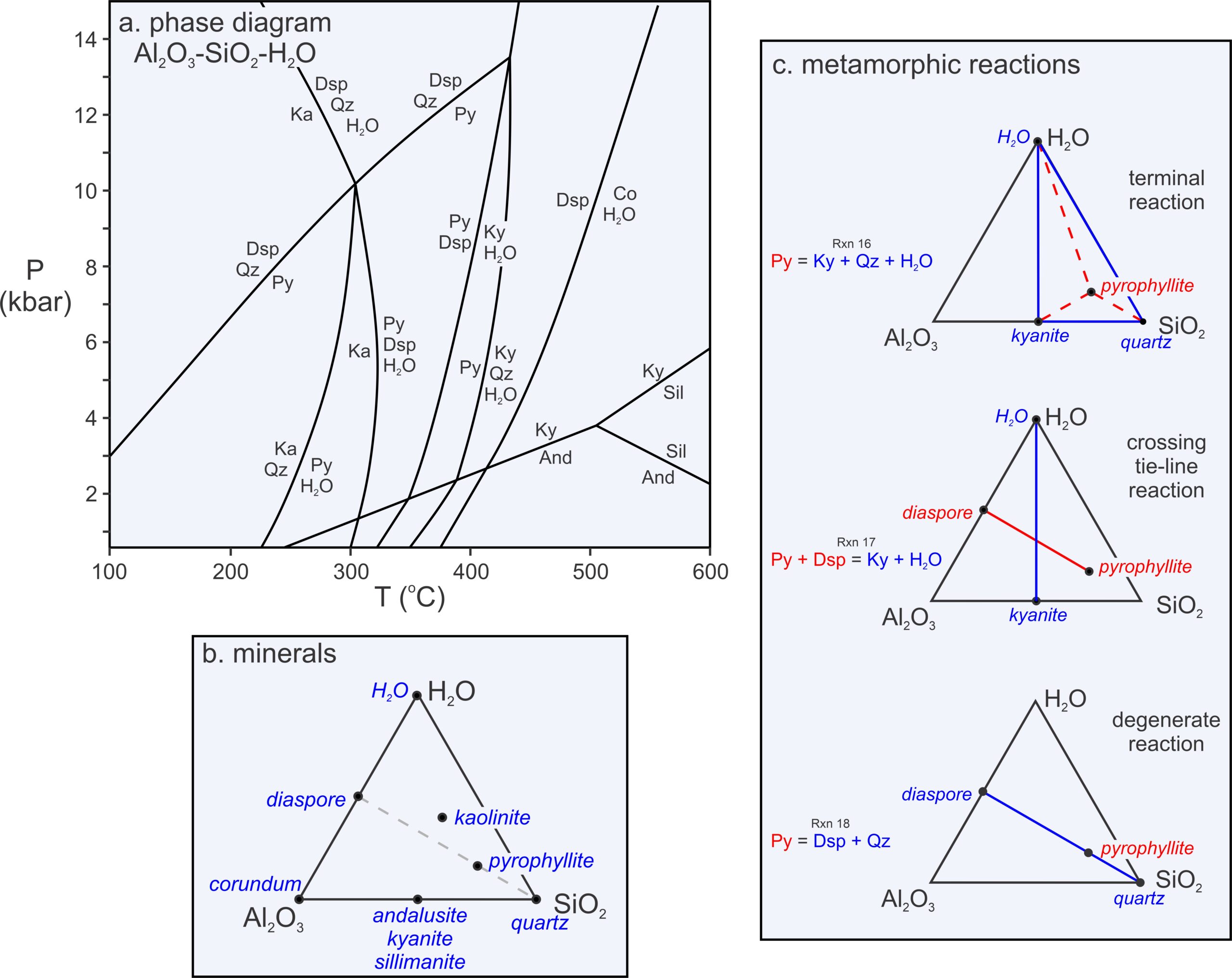
Figure 11.20c contains triangles depicting the kinds of reactions that occur in 3-component systems. Some, which we call terminal reactions (because they may cause a mineral to disappear), involve a single phase reacting to three others. The example given in Figure 11.20c (top triangle) is:
| [Rxn 8] | pyrophyllite = kyanite + 3 quartz + H2O |
This reaction involves a reactant phase (pyrophyllite) that plots in a triangle created by three other product phases (kyanite, quartz, and H2O). Terminal reactions always have this kind of configuration in triangular chemographic diagrams, but sometimes the triangle is very scalene or obtuse.
Some 4-phase reactions, however, have two phases on each side of the equal sign, such as the reaction of pyrophyllite and diaspore to kyanite and H2O:
| [Rxn 4] | pyrophyllite + 6 diaspore = 4 kyanite + 4 H2O |
This reaction, too, is depicted in Figure 11.20c (middle triangle). Reactions of this sort – with two phases on one side of the equal sign and two on the other – are crossing tie-line reactions, sometimes called tie-line flip reactions. As seen in Figure 11.20c, a tie-line connecting the reactants crosses a tie-line connecting the products, sort of like the two sticks used to make a kite.
Most net-transfer reactions in 3-component systems are terminal reactions or tie-line flip reactions, but Figure 11.20c also contains one other kind of reaction (bottom triangle) – a reaction that contains only three phases:
| [Rxn 21] | 2 diaspore + 4 quartz = pyrophyllite |
Reaction 19 is an example of a degenerate reaction in the 3-component Al2O3-SiO2-H2O system because, instead of three, we can describe it using only two components. The compositions of pyrophyllite, diaspore, and quartz all fall into the 2-component AlO(OH)-SiO2, system. We do not need a third component to describe these mineral compositions. Graphically, we can see this is the case in Figures 11.20b and 11.20c – the three minerals (pyrophyllite, diaspore, and quartz) plot on a line like phases in any 2-component system.
Notice that diaspore, corundum, and H2O all plot on the line that is the left side of the triangle in Figure 11.20b. So we can describe their compositions with only two components. Thus, the reaction of diaspore to corundum and H2O, plotted on the phase diagram in Figure 11.20a, is also degenerate in the Al2O3-SiO2-H2O system. It contains only 3 phases:
| [Rxn 9] | 2 diaspore = corundum + H2O |
Figure 11.20a also contains three doubly degenerate reactions involving kyanite, andalusite, and sillimanite (Reactions 1, 2, and 3, considered earlier in this chapter). These reactions involve only one component and only two minerals – two fewer phases than nondegenerate reactions in a 3-component system.
11.4.4 Using Triangular Composition Diagrams

Triangular composition diagrams contain much information. Most importantly, we can use them to depict possible stable mineral assemblages in different parts of P-T space. The triangle on the left in Figure 11.16 is an example – a chemographic diagram with three components (Al2O3, SiO2, H2O, labeled in red) and six phases (labeled in blue). The triangular diagram lists stable 3-mineral assemblages (labeled in black) in the low-temperature but high-pressure field on the phase diagram. Notice that all parts of the chemographic triangle are divided into small triangles connecting minerals that may coexist. There are no 4-sided areas. The phase rule requires this – it tells us that in a 3-component system, a maximum of three minerals may exist together (unless a reaction is occurring).
Consider a hypothetical rock with composition equivalent to some combination of Al2O3, SiO2, and H2O. We can plot the composition on the chemographic triangle in Figure 11.16 to learn the stable mineral assemblage at low temperature and high pressure. The diagram also tells us that if (unlikely), a rock has a composition equal to a single mineral (Co, Dsp, Ky, Qz, or Ka), the rock will contain only that mineral. If a rock has composition equivalent to some combination of two minerals, it will plot on a line in the triangle, and the rock will contain only two minerals. Most rock compositions, however, will plot within triangles, and the rocks will contain three minerals.
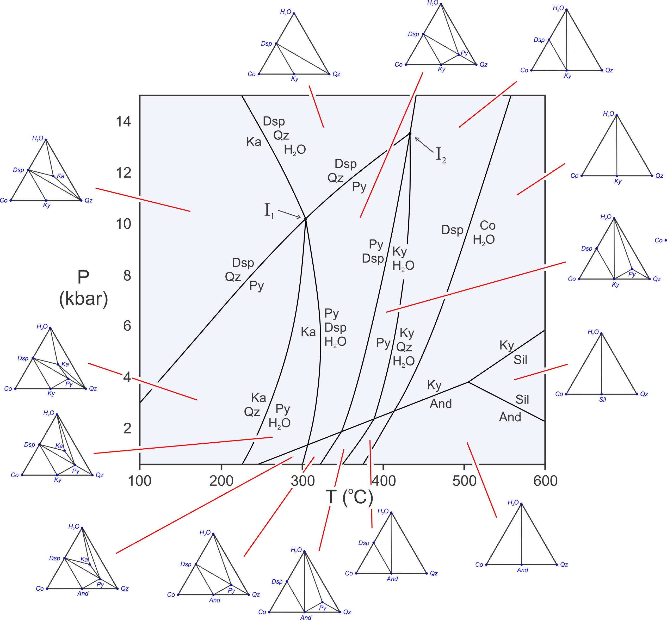
Figure 11.22 has composition triangles for all the fields on the Al2O3-SiO2-H2O phase diagram. At low temperature, hydrous phases (kaolinite, pyrophyllite, and diaspore) are stable. But, as temperature increases, one-by-one they break down. So, at the highest temperatures, only anhydrous minerals remain, and the number of possible minerals is small. The composition diagrams are different on different sides of every reaction. Either a terminal or degenerate reaction has occurred – adding or eliminating a mineral – or a crossing tie-line reaction has occurred when we cross from one field to another.
The composition diagrams show all possible three phase assemblages. They are stable in open spaces between reactions. Four phases may coexist if P-T conditions fall on a reaction line. And at invariant points, where reactions intersect, five phases may coexist. For example, at the invariant point labeled I1 in Figure 11.22, kaolinite, diaspore, quartz, pyrophyllite, and H2O may coexist. The odds of a rock equilibrating precisely at such conditions are, however, extremely small.
11.4.5 Invariant Points and Metastable Reactions
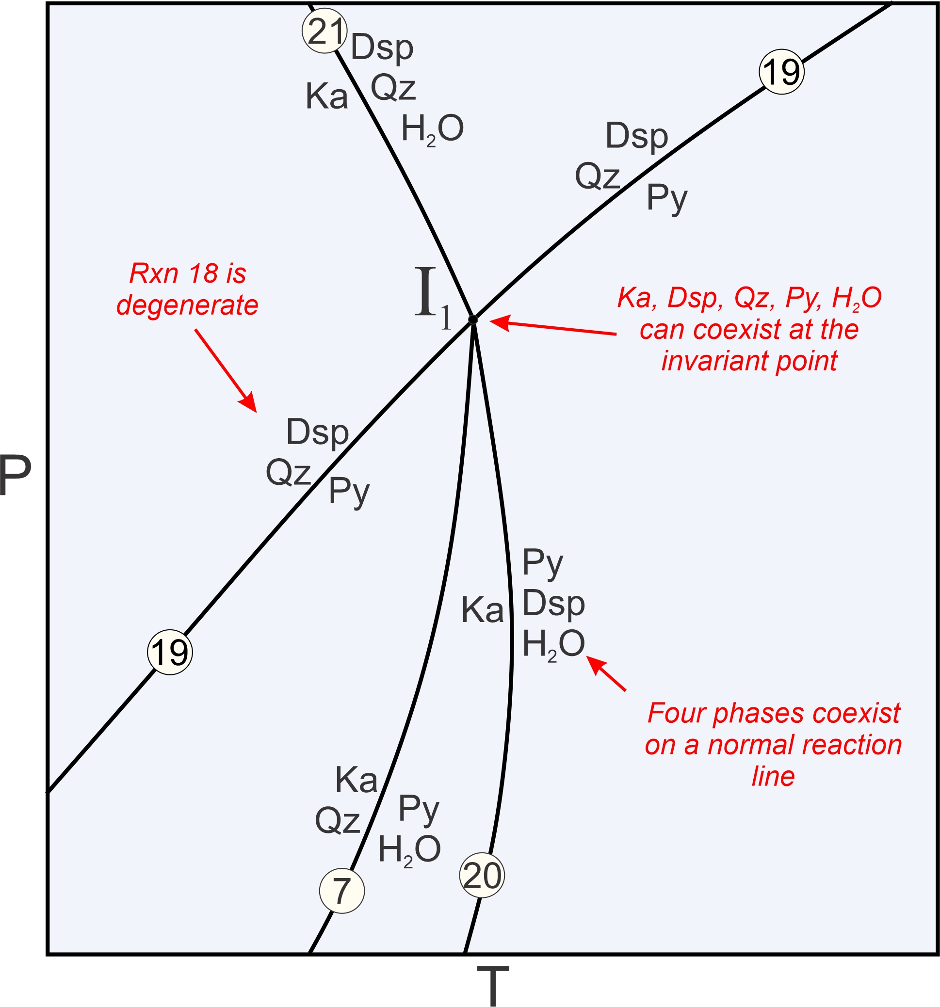
Previously we described metastable reactions as reactions that cannot take place anywhere because the phases involved are never stable together. Other kinds of metastable reactions can take place but stop at invariant points. For example, Figure 11.23 is an enlarged view of the invariant point labeled I1 in Figure 11.22. Four reactions intersect at the point where five phases can coexist (Dsp, Qz, Py, Ka, and H2O):
| [Rxn 7] | kaolinite + 2 quartz = pyrophyllite + H2O |
| [Rxn 21] | pyrophyllite = 2 diaspore + 4 quartz |
| [Rxn 22] | 2 kaolinite = pyrophyllite + 2 diaspore + H2O |
| [Rxn 23] | kaolinite = 2 diaspore + 2 quartz + H2O |
A maximum of four phases coexist along reaction curves emanating from the point. And in space between reactions, only three phases are stable together. In all, there are 12 possible assemblages involving the five phases that may be stable at some place on this diagram.
Reaction 19 is a degenerate reaction that passes through invariant point I1. The other three reactions (Reactions 7, 20, and 21, which are not degenerate) do not continue past the invariant point. Why do the reactions stop? Consider that reactions 7 and 20 involve pyrophyllite. But, the degenerate reaction (19) tells us that pyrophyllite is not stable at pressures above the invariant point. So, reactions 7 and 20 must stop there. Similarly, the degenerate reaction tells us that diaspore and quartz may not coexist at pressures below the invariant point. So, reaction 21 (which involves diaspore and quartz) stops at the point. Degenerate reactions commonly pass through invariant points while causing other reactions to become metastable, as happens in this diagram. There are, however, counterexamples.
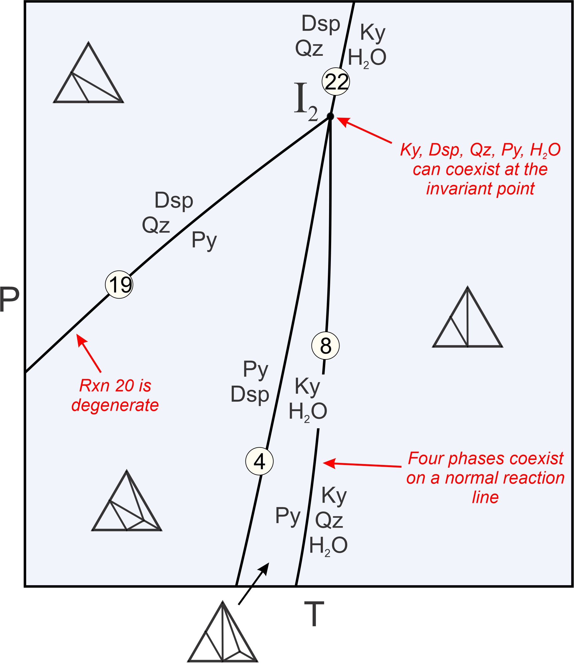
Figure 11.24 is a closeup of the other invariant point in Figure 11.22, I2. Four reactions intersect at I2 where five phases can coexist:
| [Rxn 4] | pyrophyllite + 6 diaspore = 4 kyanite + 4 H2O |
| [Rxn 8] | pyrophyllite = kyanite + 3 quartz + H2O |
| [Rxn 21] | 2 diaspore + 4 quartz = pyrophyllite |
| [Rxn 24] | 2 diaspore + quartz = kyanite + H2O |
In contrast with I1, all of the reactions involved stop at I2. As with I1, five phases can coexist at this point and normal reactions involve four phases. Reaction 19, the same degenerate reaction that passed through point I1, ends at I2. It becomes metastable there because pyrophyllite, and also an assemblage of diaspore + quartz, cannot exist at temperatures greater than I2 because of the other reactions that take place. Box 11.3 discusses in more detail how reactions intersect at invariant points I1 and I2.
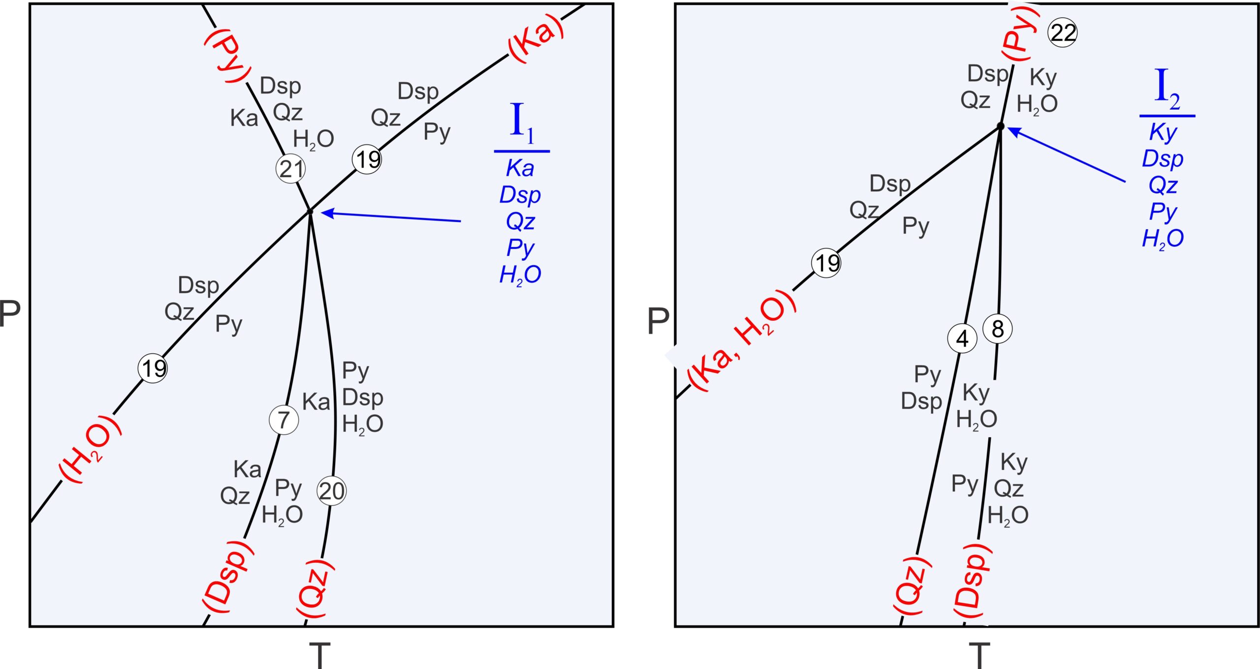
● Box 11.3 The Phase Rule, Algebra, and an Alternative Way to Label Reactions at Invariant Points
space Five phases coexist at each invariant point (listed in blue): kaolinite, diaspore, quartz, pyrophyllite and H2O at I1. I2 contains the same minerals except that kyanite replaces kaolinite. For a bundle of reactions that intersect at an invariant point, each phase must be missing from one (and only one) reaction. The missing phases for each reaction are in red parentheses in the table below, and in red labels on each reaction curve in the phase diagrams above in Figure 11.25. Degenerate reactions such as Reaction 19 always lack more than one phase. In the drawing of invariant point I1 (on the left), the missing H2O and Ka are put on opposite extensions of the Reaction 19 curve, as is conventionally done. In the drawing on the right, Reaction 19 terminates at I2, so we list both missing phases together.
We can manipulate reactions algebraically. For example, we can add or subtract any two to eliminate a phase and get another reaction that passes through the same invariant point. This explains why every phase will be missing from one reaction. The invariant points depicted in Figure 11.25 above depict two ways that reactions may interact at an invariant point. Sometimes reaction curves continue through invariant points, and sometimes not. There are many possible variations depending on the number of components and on phase compositions. For multicomponent systems we can use the Schreinemakers’ Method to determine the relationships of curves around any invariant point. We can apply this method to a variety of phase diagrams. For a summary, go to Method of Schreinemakers — A Geometric Approach to Constructing Phase Diagrams at https://serc.carleton.edu/research_education/equilibria/schreinemakers.html. |
11.5 Systems With More than Three Components and Projections
Systems with more than three components can be very complex. One problem is that we cannot construct two-dimensional chemographic diagrams to describe mineral compositions. Another complication is that there may be many reactions, and most involve five or more phases. So phase diagrams become cluttered and hard to read. Additionally, we can often predict and interpret mineral equilibria by considering only a smaller number of components, which means we may not need to consider more complicated systems. Nonetheless, sometimes we wish to look at systems with more than three components. Suppose we want to consider a 4-component system. To do this graphically and to construct triangular two-dimensional chemographic diagrams, we could decide to ignore a component.
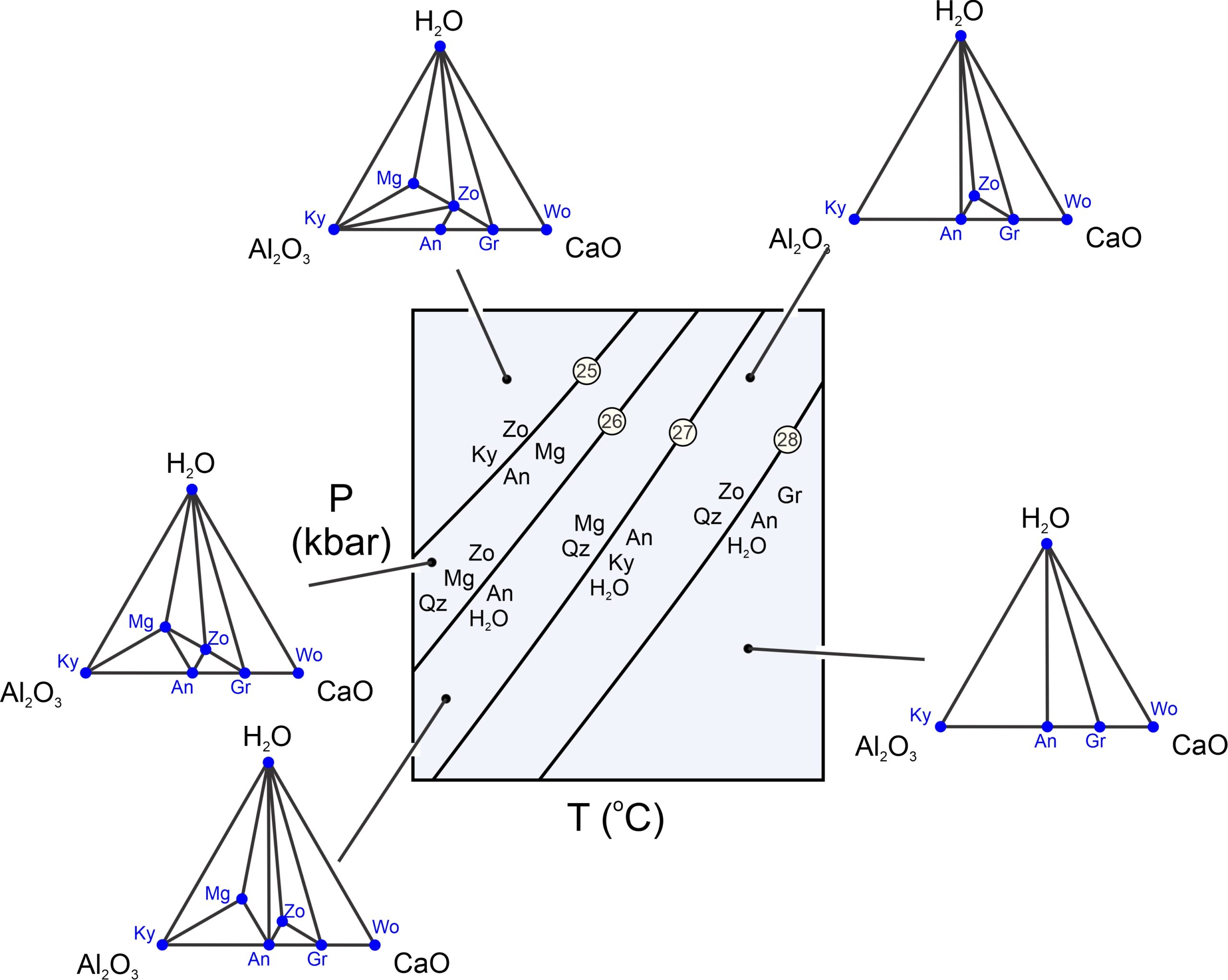
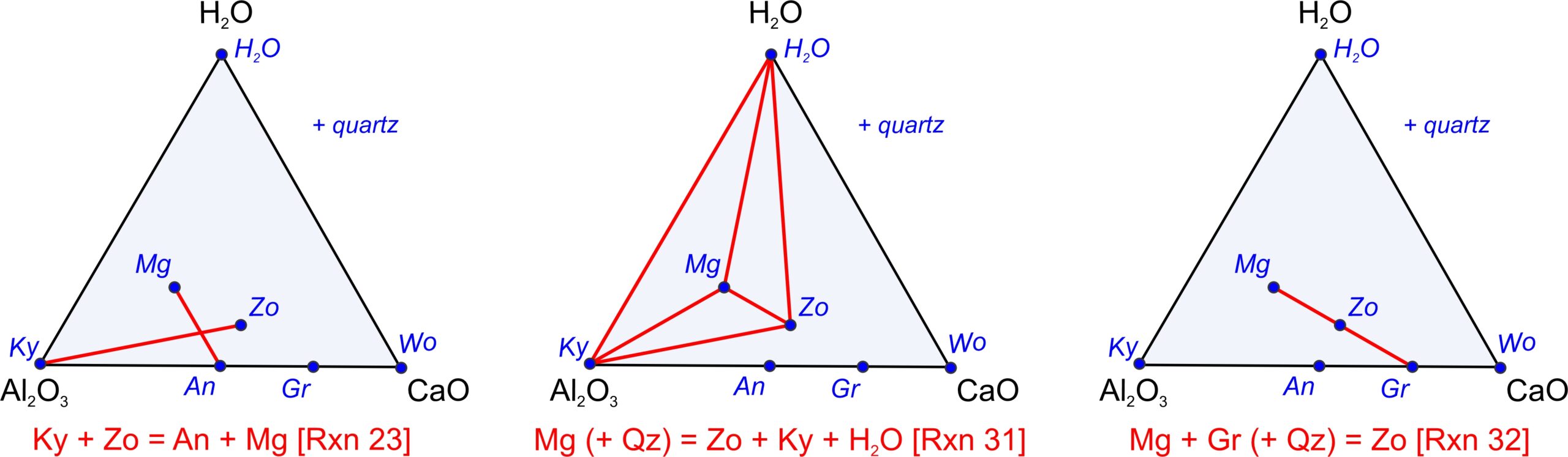
Consider hypothetical rocks in the 4-component CaO-Al2O3-SiO2-H2O system. These rocks might contain some combinations of grossular, quartz, kyanite, zoisite, margarite, wollastonite, anorthite, and H2O. Figure 11.26 includes some low-temperature reactions that can affect such rocks. Typical reactions involve five phases, but degenerate reactions involve fewer.
The reactions in Figure 11.26 are:
| [Rxn 25] | 2 Ky + 2 Zo = 3 An + Mg |
| [Rxn 26] | 2 Zo + Mg + 2 Qz = 5 An + 2 H2O |
| [Rxn 27] | Mg + Qz = An + Ky + 2 H2O |
| [Rxn 28] | 4 Zo + Qz = Gr + 5 An + 2 H2O |
Rocks containing combinations of grossular, kyanite, zoisite, margarite, wollastonite, or anorthite often contain some quartz, so let’s assume it is present and ignore the SiO2 component of the minerals. We make projections by plotting the mineral compositions on chemographic triangles after subtracting the SiO2 that they contain. The triangular diagrams in Figure 11.26 then, are projected from quartz. We can always project from a mineral, in this example quartz, to show potential mineral reactions in a rock – provided the mineral will always be present. This means, for a 4-component system, we can eliminate a component and construct two-dimensional chemographic triangles.
Reactions 25 and 26 in Figure 11.26 appear as tie-line flip reactions (two minerals replace two others, ignoring quartz) in the chemographic projections. Reactions 27 and 28 appear as terminal reactions (that eliminate a mineral) in Figure 11.26. We can see these relationships in the triangles because we used a projection. If we did not project, we would have to look at three-dimensional chemographic diagrams which are difficult to see (and to construct). The triangular chemographic diagrams in Figure 11.26 obey the phase rule for a 3-component system. The triangles show a maximum of three phases may coexist for any composition. Four phases could coexist when a reaction is occurring. However, because we projected from quartz (not plotted as a point in the triangular diagrams), quartz is stable for all compositions. If quartz was not stable for all compositions, we would find inconsistencies in our triangles. Either we would get four-mineral regions (instead of triangles), or we would get inconsistent or crossing tie lines when we looked at natural examples.
11.5.1 More About Projections
What happens when we project from a mineral? The fundamental change is that we reduce the number of components. The example we just considered involved phases in the CaO-Al2O3-SiO2-H2O system. By projecting from quartz, we eliminated SiO2 and could plot the minerals on a CaO-Al2O3-H2O triangle.
Let’s look at other examples of projections. We will start with a relatively simple projection from two dimensions (a 3-component triangle) to one dimension (a 2-component line). Figure 11.27 is an example involving five minerals in the CaO-Al2O3-SiO2 system (kyanite, anorthite, grossular, wollastonite, and quartz).
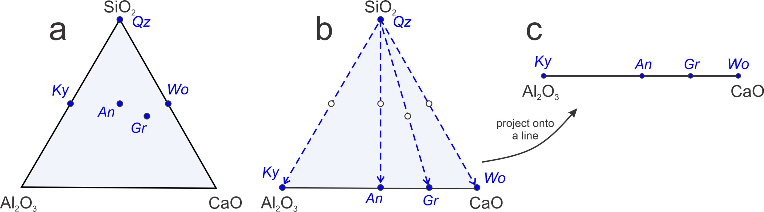
Figure 11.27a shows the mineral compositions plotted on a 3-component (ternary) diagram. Figure 11.27b shows (with blue dashed arrows) how we can project those mineral compositions (from quartz, SiO2) onto the base of the triangle. The result is the pseudobinary Al2O3-CaO diagram in Figure 11.27c. It is a pseudobinary, not a true binary, because the minerals plotted have compositions that include SiO2 (which is not part of the diagram) besides Al2O3 and CaO. Note that quartz does not plot on this binary. The projection from quartz allows us to plot compositions on a line and is appropriate for describing equilibria involving kyanite, anorthite, grossular, wollastonite, provided quartz is present.
As we saw previously, binary diagrams allow us to identify reactions involving any three minerals. Given any three minerals that plot on a line, we can always balance a reaction involving the two minerals on the outside reacting to create the one between them. Thus, for the system seen in Figure 11.27c, four possible pseudobinary reactions (with projected Qz in blue) are:
| [Rxn 29] | An = Ky + Wo |
| [Rxn 30] | 3 An = 2 Ky + Gr (+Qz) |
| [Rxn 31] | An + 2 Wo = Gr (+Qz) |
| [Rxn 32] | Ky + 3 Wo = Gr (+Qz) |
Reaction 29 is degenerate and we can balance it with just the three minerals listed (they fall on a line in Figure 11.27a). Reactions 30, 31, and 32, however, cannot be balanced without adding quartz to the right-hand side. That is why projecting from quartz requires quartz to be present.

Petrologists do not normally project from triangles to lines because triangular diagrams are usually quite easy to interpret, and they contain information lost with a projection. But, petrologists do commonly project from systems with more than three components to reduce the number of components and allow construction of two-dimensional drawings. Figure 11.28 is an example of projecting from a 4-component system (a tetrahedron) to a 3-component system (a triangle).
Figures 11.28a and 11.28b show compositions of some minerals in the CaO-Al2O3-SiO2-H2O system. They plot as dots on and within a CaO-Al2O3-SiO2-H2O tetrahedron. The minerals in Figure 11.28a (kyanite, quartz, anorthite, grossular, and wollastonite) are anhydrous and so plot on the front-left face of the pyramid. The minerals in Figure 11.28b (margarite and zoisite) contain all four components and so plot within the pyramid.
To reduce the number of components to three, and the number of dimensions to two, we can project from quartz (shown by blue dashed arrows in Figures 11.28a and 11.28b). The result is a pseudoternary triangular diagram (Figure 11.28c). The “+quartz” (in the box in Figure 11.28c) reminds us that we projected from quartz and, because we projected from quartz, quartz does not plot on the triangle. Kyanite, anorthite, grossular, and wollastonite project to the bottom edge of the triangle, plotting between Al2O3 and CaO, because they are anhydrous. The hydrous minerals (margarite and zoisite) plot in the triangle’s interior.
We can use the pseudoternary diagram in Figure 11.28c to identify reactions involving any of the minerals. Because we projected from SiO2, quartz may be involved as a reactant or product although it does not plot on the diagram. Figure 11.29 depicts some example reactions. Figure 11.29a depicts a tie-line flip reaction, Figure 11.29b depicts a terminal reaction, and Figure 11.29c depicts a degenerate reaction. These reactions are:
| [Rxn 25] | 2 Ky + Zo = 3 An + Mg |
| [Rxn 33] | 4 Mg (+3 Qz) = Zo + Ky + H2O |
| [Rxn 34] | Mg + Gr (+ Qz) = 2 Zo |
We can balance Reaction 25 without quartz. The second two reactions do not balance without quartz on the left side. (But, that is OK because we projected from quartz.) Reaction 33, with quartz added on the left side, contains five phases, consistent with the phase rule for a 4-component (CaO-Al2O3-SiO2-H2O) system. Reactions 25 and 34 are degenerate, containing four phases only.
11.5.2 ACF Diagrams
The hypothetical system we just considered contained four components – and it involved a complicated projection. Most common natural rocks contain seven or eight, and generally more, important components. If you look up the analysis of a typical rock, for example, you may see as many as 12 components listed, perhaps these: SiO2, Al2O3, FeO, Fe2O3, CaO, Na2O, K2O, MgO, MnO, TiO2, P2O5, and H2O. Some of these may be insignificant sometimes, but 12 is many more than we can consider if we wish to construct chemographic diagrams – three components is the most we can depict in two-dimensional drawings.
In the early 1900s, Pentti Eelis Eskola, a Finnish geology professor, developed methods for reducing complex multicomponent systems to three so he could plot mineral compositions and reactions on triangular diagrams. Following Eskola’s lead, petrologists today use the following approaches to “eliminate” components and reduce the number of compositional dimensions:
1. We can combine components. For example, Fe, Mg, and Mn substitute for each other in many solid-solution minerals. So, we can think of FeO, MgO, and MnO as one pseudocomponent. We abbreviate this component F. We also commonly think of Al2O3 and Fe2O3 as a single pseudocomponent (which we designate A) because most rocks contain little Fe2O3 and because Al3+ and Fe3+ enter the same minerals and behave about the same in many rocks.
2. We can ignore components. For example, some rocks contain small amounts of phosphorous. If a rock contains phosphorous, it generally contains the mineral apatite, Ca5(PO4)3(OH). Phosphorous is rarely found in other minerals, so phosphorous does not generally take place in reactions during metamorphism. Unless considering very uncommon rocks, we simply ignore apatite and any P2O5 component a rock may contain. We sometimes ignore Fe2O3, TiO2 and other components for similar reasons.
3. We can project from components that are in excess and always present. We saw examples of this earlier in this chapter when we projected from SiO2 and we will see more examples below.
In 1915, Eskola presented what we now call the ACF diagram as a way to plot mineral assemblages on triangular diagrams. Eskola initially considered 11 components: SiO2, Al2O3, Fe2O3, CaO, FeO, MgO, MnO, Na2O, K2O, P2O5, and H2O. To reduce the number of components, Eskola combined FeO, MgO, and MnO into one pseudocomponent (F). He combined Al2O3 and Fe2O3 into another pseudocomponent (A), and considered CaO (C) as the third component. The nominal values for the three components then are:
A = moles of Al2O3 and Fe2O3 combined
C = moles of CaO
F = moles of FeO, MgO, and MnO combined
To handle the SiO2, Na2O, K2O, P2O5, and H2O, Eskola projected compositions from albite, orthoclase, quartz, apatite, and H2O, eliminating five components as follows:
• Eskola recognized that most Na2O and K2O in common rocks is in alkali feldspars, and that these components rarely have a major effect on mineral reactions. So, in ACF diagrams, he projected compositions from albite (NaAlSi3O8) and orthoclase (KAlSi3O8). This means he subtracted any albite or orthoclase component from the overall rock composition and from mineral compositions. Essentially, he was pretending the feldspar components were unimportant while eliminating Na2O and K2O from further consideration. Because feldspars contain Al2O3, and because Eskola was projecting from feldspars, he subtracted the Al2O3 in feldspars from the A component. Feldspars contain one mole of Al2O3 for every mole of Na2O and K2O, so (subtracting feldspar Al2O3) a revised value for A is:
A = Al2O3 + Fe2O3 – Na2O – K2O
• Similarly, Eskola projected from apatite. Projecting from apatite means that the P2O5 is eliminated from further consideration. Apatite contains 3.33 moles of CaO for every mole of P2O5. Because of the projection, that amount of CaO is subtracted from the value for C:
C = CaO – 3.33 P2O5
• Eskola also projected from SiO2 and H2O, which is tantamount to assuming that quartz and H2O are always present. (This assumption is not valid for all rocks but generally does not lead to significant problems or contradictions.)
So, for Eskola’s ACF diagram we have these three components:
A = Al2O3 + Fe2O3 – Na2O – K2O
C = CaO – 3.33 P2O5
F = FeO + MgO + MnO
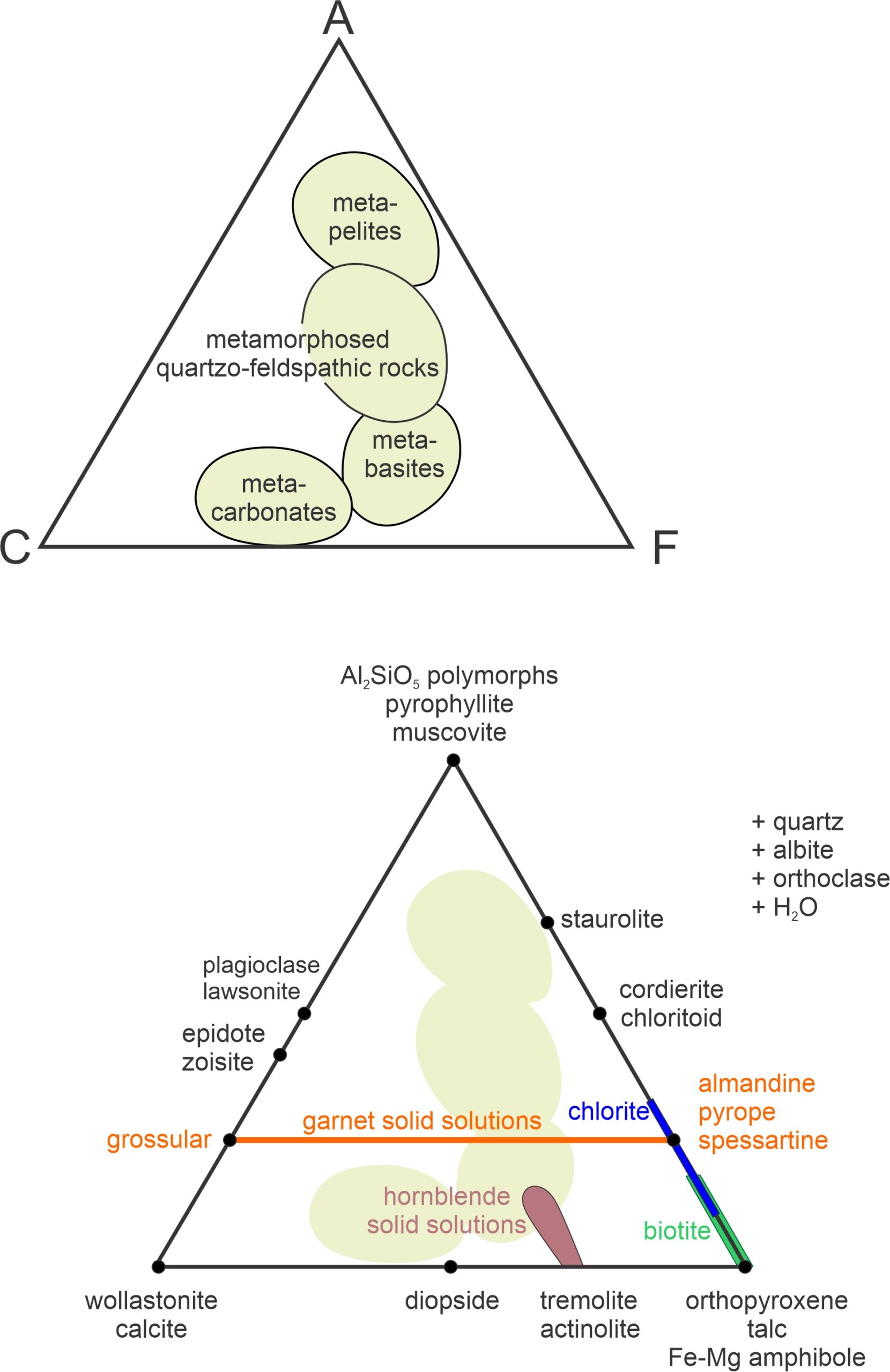
Calculating values for A, C, and F is based on the moles of oxides present. We use the equations above to get values, normalize the results to 100%, and can plot the results on an ACF diagram. Figure 11.30 contains examples. The top triangle shows where rocks of different composition plot. Metapelites (equivalent to metamorphosed clay-rich sediments) plot near the A corner because they are Al2O3-rich. Metabasites, such as metabasalt or metagabbro plot closer to the F corner (they are relatively FeO- and MgO-rich). Metacarbonates, which usually contain little Al2O3, plot near the bottom edge between C and F. And quartzofeldspathic rocks, such as metagranites or metamorphosed feldspathic sandstone, plot near the center of the diagram.
The bottom triangle in Figure 11.30 shows where some common metamorphic minerals plot on an ACF diagram. Minerals with a fixed composition are plotted as (black) points. Minerals that form solid solutions plot on a line, or in an area. In Figure 11.30, an orange line depicts possible garnet compositions. They range from pure grossular (Ca-garnet) to almandine-pyrope-spessartine (Fe-Mg-Mn garnet) which all plot at the same point on the other side of the triangle. Natural hornblende compositions plot in a brown blobby area, but are anchored by Al2O3-free tremolite and actinolite on the bottom edge of the triangle. Biotite (green line) and chlorite (blue line) are solid-solution minerals that generally contain little CaO, but contain variable amounts of Al2O3. So, they plot as lines on the right side of the triangle. ACF diagrams are projected from quartz, albite, orthoclase, and H2O, indicated by +quartz, +albite, +orthoclase, and +H2O (to the right of the triangle).

Figure 11.31 is an ACF diagram for medium-grade metamorphic rocks in Scotland’s Highlands. The diagram, based on a classic 1981 study by Francis Turner, shows stable mineral assemblages for one specific pressure and temperature. If P-T conditions changed significantly, the minerals present, the fields, or the tie-lines would also change. If we know a rock’s composition, we can calculate A, C, and F using the equations above. We then use the values to plot the composition on the ACF diagram to learn the ACF minerals that will be present in the rock. Some composition rocks will contain three ACF minerals (if they have compositions that plot in one of the blue triangular fields), and some fewer. If a composition plots in one of the white regions that contains subparallel lines, for example, only two ACF minerals will be present. But because this diagram is projected from SiO2, NaAlSi3O8, KAlSi3O8, and H2O, it is tacit that all composition rocks will contain quartz, alkali feldspar, and H2O besides the ACF minerals labeled within the fields.
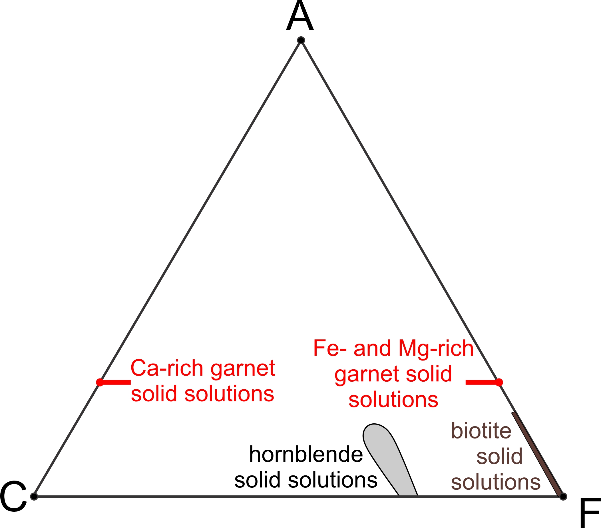
Several minerals in Figure 11.31 are solid solutions and thus have a range of possible compositions. Figure 11.32 shows ranges of the solid-solution compositions more clearly. Two short red lines represent possible garnet compositions. Garnet may be calcium-rich or calcium-poor (rich in iron and magnesium instead). Biotite may contain some aluminum, and a brown line from the F apex extending part way toward A shows possible biotite compositions. A gray blob near the bottom of the diagram shows possible hornblende compositions. But, hornblende has more variations in composition that cannot be plotted on this diagram. The other minerals depicted in Figure 11.31 have compositions that plot as points on this diagram because they do not vary.
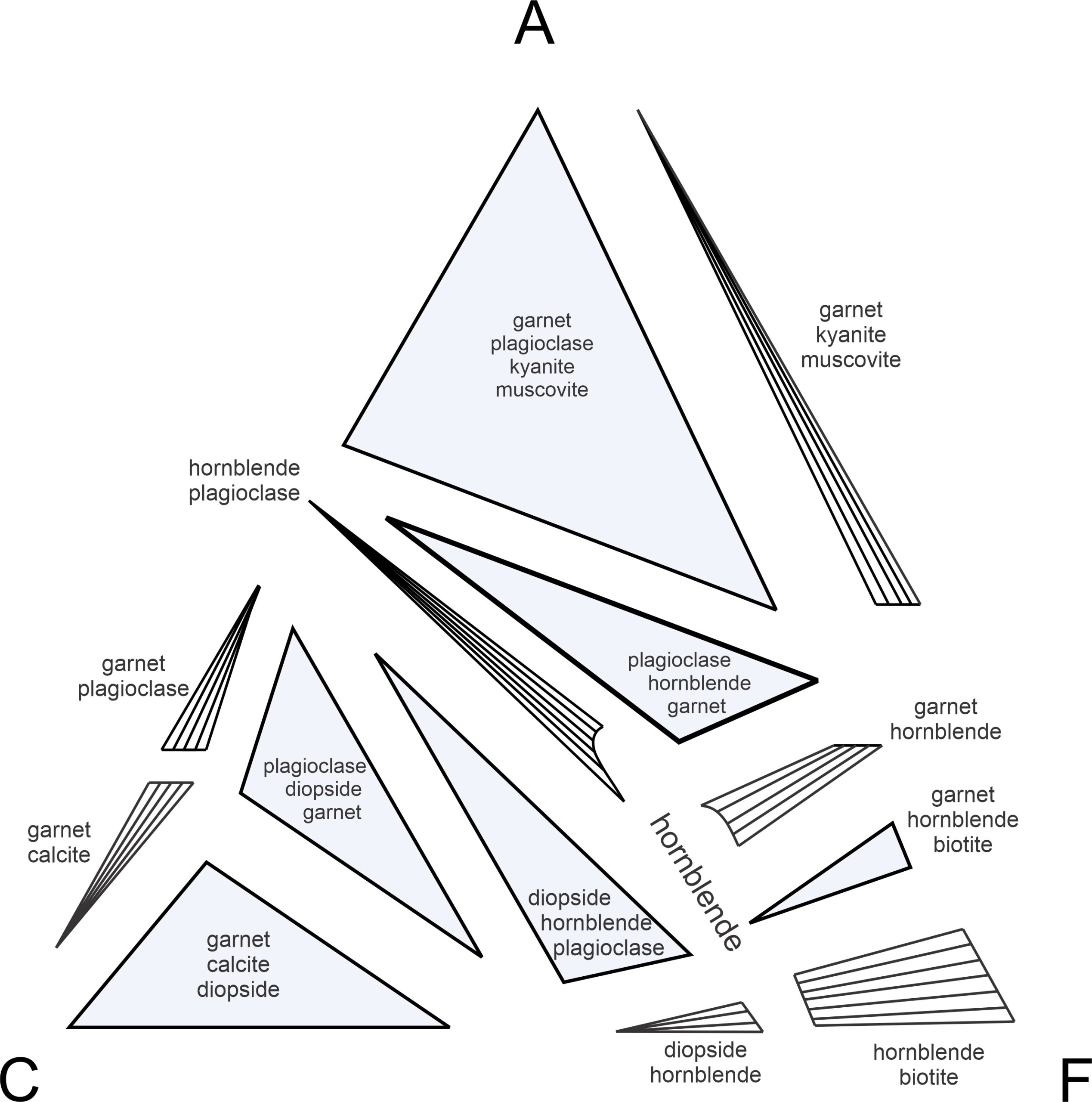
Figure 11.33 is an exploded view of the same ACF diagram in Figure 11.31. It displays more clearly that rock compositions may plot into triangular 3-phase fields where three ACF minerals can coexist (shaded blue), or may plot into other regions (white with subparallel tie lines) where only two ACF minerals will coexist. The tie lines in the white 2-phase fields connect two mineral compositions that coexist. If a rock composition happens (unlikely) to be the same as a single ACF mineral composition, it will contain only that ACF mineral.
Diagrams like the one in Figure 11.31 (and Figure 11.33) remind us why chemographic projections are informative and useful. The diagram gives an immense amount of information – all the possible mineral assemblages for rocks of different compositions – that would be hard to describe concisely with words alone.
The triangular diagrams we just looked at show stable mineral assemblages over a limited range of pressure-temperature conditions. Still, in principle we can construct ACF diagrams that describe the stable assemblage for any conditions. In practice, however, we sometimes run into problems. The biggest problems stem from the assumptions made when constructing the diagram. When creating ACF diagrams, we combine some components, which implies they always behave the same way. We also projected from some phases, which implies they are always present. These assumptions are valid for some rocks, most of the time, but not for all rocks all of the time. Thus we may get contradictions – for example we may find minerals coexisting that are unconnected by tie lines, or we may find too many minerals coexisting. The trick, then, is to find the best kind of diagram to use for rocks of different compositions. If a diagram works perfectly, it will be consistent with the phase rule for a 3-component system.
11.5.3 Eskola’s AFM Diagrams for Pelites
Eskola recognized that ACF diagrams do not apply particularly well to pelites. For example, the top triangle in Figure 11.31 contains four minerals – which violates the phase rule for a 3-component system. And, the minerals in the bottom of the ACF triangle (calcite, diopside, and hornblende) are not commonly found in pelites. To solve these problems, Eskola derived a different kind of projection.
Eskola noted that Al2O3, K2O, FeO, and MgO are the most important components in pelites. To show these components in three dimensions, Eskola constructed a pyramid with the following components at the corners:
A = Al2O3 – Na2O – K2O – CaO
K = K2O
F = FeO
M = MgO
As with the ACF diagram, in the AKFM pyramid he projected mineral compositions from SiO2 and H2O. He also projected from albite (NaAlSi3O8), orthoclase (KAlSi3O8), and anorthite (CaAl2Si2O8). Thus, he subtracted Na2O, K2O, and CaO from A, so the value of A only reflected the Al2O3 that is not in feldspars.
The components in the AKFM pyramid are quite similar to the ones used for the ACF diagram already discussed, except that FeO and MgO are separated. (For simplicity, here and in the rest of this chapter, we will disregard components Fe2O3 and P2O5, but we could include them without changing anything of significance.)
Figure 11.34 contains two views of an AKFM tetrahedron. The pyramid on the left shows the compositions of some Al-, Fe-, and Mg-containing minerals that are common in metapelites. They plot on the front face of the AKFM pyramid because they contain no K2O. Because their compositions range from Fe-rich to Mg-rich, they plot as lines. The line for chlorite is wider than the others because chlorite contains somewhat variable amounts of Al2O3.
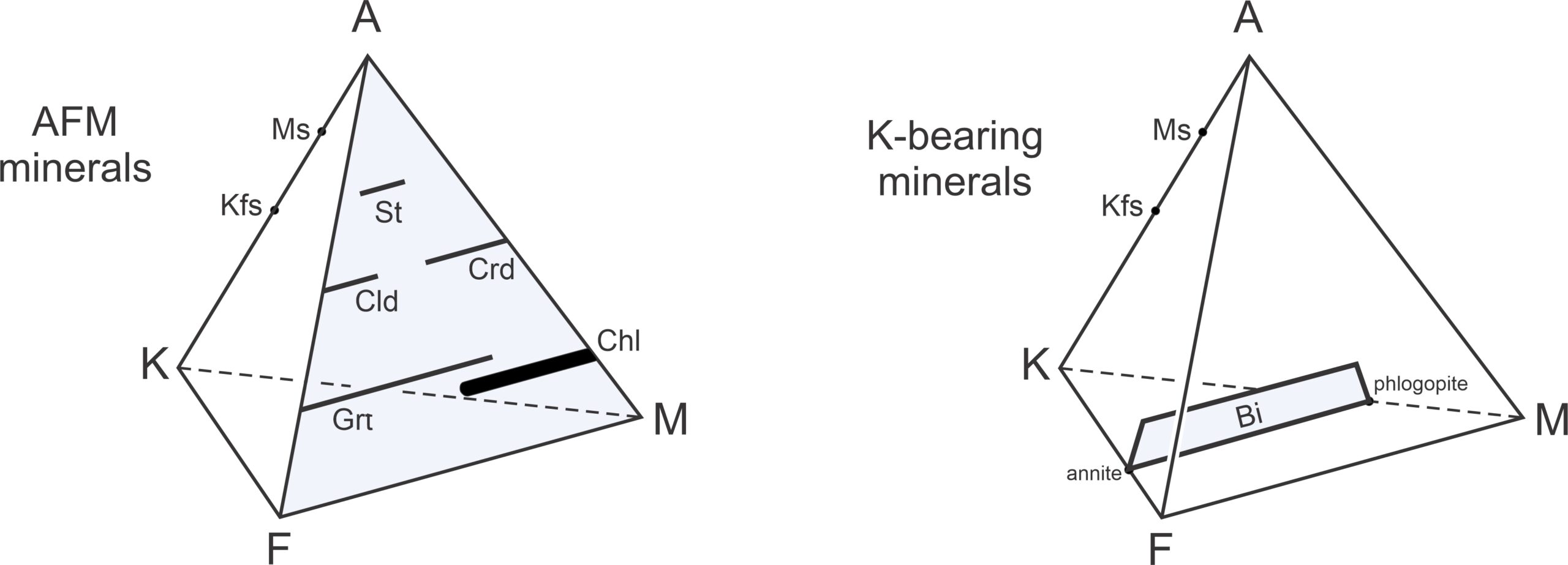
The pyramid on the right in Figure 11.34 shows muscovite (Ms) and K-feldspar (Kfs), both potassium-aluminum silicates, plotting on the back edge of the pyramid between the A and K apices. This figure also shows possible compositions of biotite. Biotite ranges from phlogopite (Mg-biotite) to annite (Fe-biotite) but also may contain variable amounts of aluminum. So, it plots as an area – a band within the pyramid’s interior.
A problem with Figure 11.34 is, of course, that the AKFM pyramid is 3-dimensional. Because so many phases plot on the AFM face, it is tempting to project from the K apex onto the AFM face to get to two dimensions. Eskola and others, however, realized that this would not work because we can only project from a phase that is always present, and no phase corresponds to K2O. (We won’t go into specifics, but projection from K2O leads to tie lines and assemblages inconsistent with natural assemblages.)
Eskola’s solution was to combine FeO and MgO to get what we call an AKF diagram. In AKF diagrams, projection from albite and anorthite accounts for all the Na2O and CaO in a rock. K2O remains as a third component). Thus:
A = Al2O3 – Na2O – K2O – CaO
K = K2O
F = FeO + MgO

Figure 11.35 shows where common metapelite minerals plot on an AKF diagram. Muscovite sometimes contains a phengite component, which means it contains variable amounts of Fe and Mg, and so plots as a sloping bar. Similarly, biotite (compositions plotted in brown) may contain Al, and so also plots as a sloping bar. Chlorite (blue) forms solid solutions with variable amounts of Al, Fe, and Mg. (Recall that in this diagram, FeO and MgO are combined to produce F.) Stilpnomelane (in green) is generally quite Fe-rich but may contain aluminum.
Figure 11.36 depicts stable mineral assemblages at low-grade, where chlorite is stable. The diagram contains white triangular fields labeled with 3-mineral assemblages. It also contains unlabeled 2-mineral fields (containing subparallel lines). In those fields, the lines connect two mineral compositions that coexist. As with other diagrams seen in this chapter, the chemographic diagram in Figure 11.36 is only valid for a particular pressure and temperature. If conditions changed significantly, the minerals present, the fields, or the tie-lines would change.
Notice that in AKF diagrams, the most important minerals in metapelites plot in different places. In the ACF diagram seen earlier, muscovite and Al2SiO5 minerals (very common in metapelites) plotted in the same spot. In AKF diagrams, they do not. Furthermore, K-feldspar, which is always present in metapelites, does not plot on an ACF diagram, but does on an AFM diagram (at the K corner). anchor
11.5.4 Thompson Projections
In 1957, some 40 years after Eskola proposed the AKF diagram, J.B. Thompson came up with a better idea. Thompson started with five components: SiO2, Al2O3, K2O, FeO, and MgO. He ignored minor components in pelitic rocks, including CaO, Na2O, and Fe2O3. Because quartz is found in all pelites, he projected from SiO2 to get the AKFM pyramid (Figure 11.34) just as Eskola did. But Thompson proposed keeping FeO and MgO as separate components. He noted that combining FeO and MgO was a mistake because the amount of FeO and MgO in a rock often determines the minerals that are present. For example, Mg-rich rocks tend to contain cordierite or chlorite, while Fe-rich rocks more often contain staurolite, chloritoid, or garnet.
To reduce three dimensions to two, Thompson suggested projecting all phases from muscovite onto the AFM face. His logic was sound because muscovite is nearly always present in metapelites. Thompson projections, also called AFM projections, work well for most metapelites and rarely lead to violations of the phase rule.
Projecting from muscovite leads to some interesting complications – perhaps that is why nobody had proposed it before Thompson. Figure 11.37 (the same pyramids seen in Figure 11.34) shows where the most important pelitic minerals plot in an AKFM pyramid, and Figure 11.38 shows the geometry of Thompson projections. All common pelitic minerals, except K-feldspar and biotite, are AFM minerals (they contain no K2O). Consequently, they do not move by projection from muscovite because they already plot on the AFM face of the tetrahedron – seen (blue) in the drawing on the left in Figure 11.37. Biotite, muscovite, and K-feldspar are different (drawing on the right in Figure 11.37).
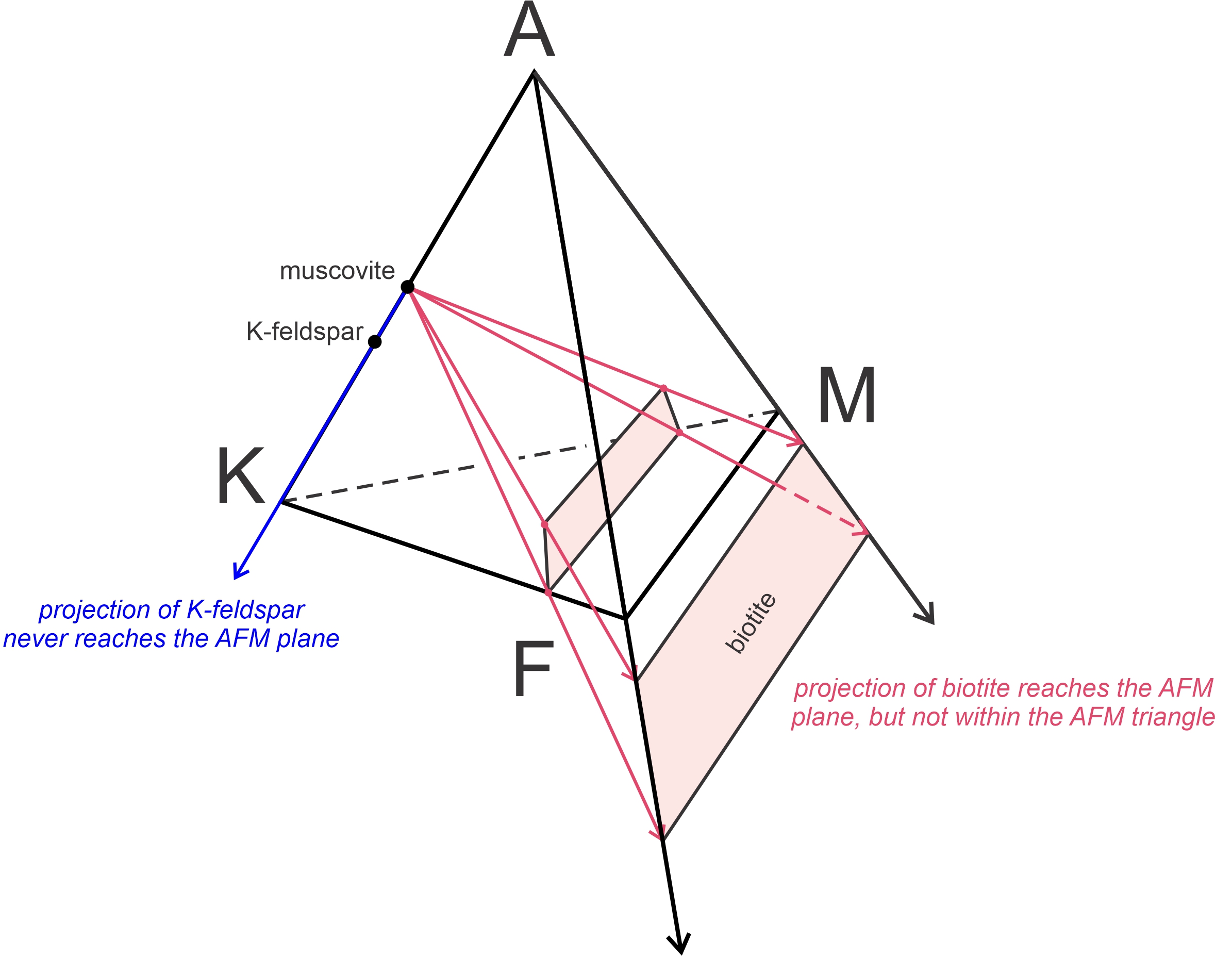
Biotite, which has compositions that plot within the AKFM tetrahedron and near its KFM base, projects to negative values of Al2O3 (red arrows in Figure 11.38). Thompson was the first person to realize that it did not matter if projecting biotite onto the AFM plane put it outside the AFM triangle. The point of projecting is to go from three dimensions to two, and that is accomplished even if A values are negative. Thompson also noted that K-feldspar, when projected from muscovite (blue arrow in Figure 11.38), projects away from the AFM plane which is equivalent to it being at infinity in the negative A direction.

Figure 11.39 shows compositions of all common pelitic minerals on a Thompson projection. The AFM minerals on the front of the pyramid in Figure 11.37 plot within the AFM triangle. Solid solution minerals that contain variable amounts of Fe and Mg (such as staurolite, chloritoid, and garnet) plot as horizontal lines. Chlorite, because of its variable Al-content, plots as a band instead of as a line. Biotite, which has a negative A value, plots in a band below the line connecting F and M. K-feldspar plots at infinity in the negative A direction (indicated by an arrow pointing down). Because this diagram is projected from muscovite and quartz, they do not plot and are assumed to be present. Rock compositions, which always plot initially within the AKFM tetrahedron will project onto the AFM plane, but may have negative values of Al2O3, like biotite does.
Looking at 3-dimensional projections and projecting them onto the front of a tetrahedron is challenging. Instead, we usually skip the 3-d step and use equations to plot compositions directly on the AFM plane. We are projecting from muscovite. So, the value of A is adjusted downward by subtracting aluminum that is in muscovite, leaving a value that reflects only the aluminum that is in other minerals. Because muscovite contains three aluminum atoms for every potassium atom:
A = Al2O3 – 3 K2O
The F and M values are just the moles of FeO and MgO:
F = FeO
M = MgO
Plotting compositions that have positive values of A, F, and M is straightforward. They plot within the AFM triangle. If the value of A is negative, however, things are not quite so simple. Consider, for example, Fe-biotite (annite), KFe3(AlSi3)O10(OH)2. For annite, using the equations above:
A = 0.5 – (3 x 0.5) = -1
F = 3
M = 0
Normalizing, we find that
%A = 100 x -1/(-1+3) = -50%
%F = 100 x 3/(-1+3)= 150%
%M = 0
The percentages above add to 100%, as they should, but one value is negative. We can do a similar calculation for phlogopite (Mg-biotite). The two mica end members (annite and phlogopite) then plot as seen in Figures 11.39 and 11.40. Solutions between the end members fall on a line between them, and if the biotite contains Al, it plots in the gray band in the diagram.
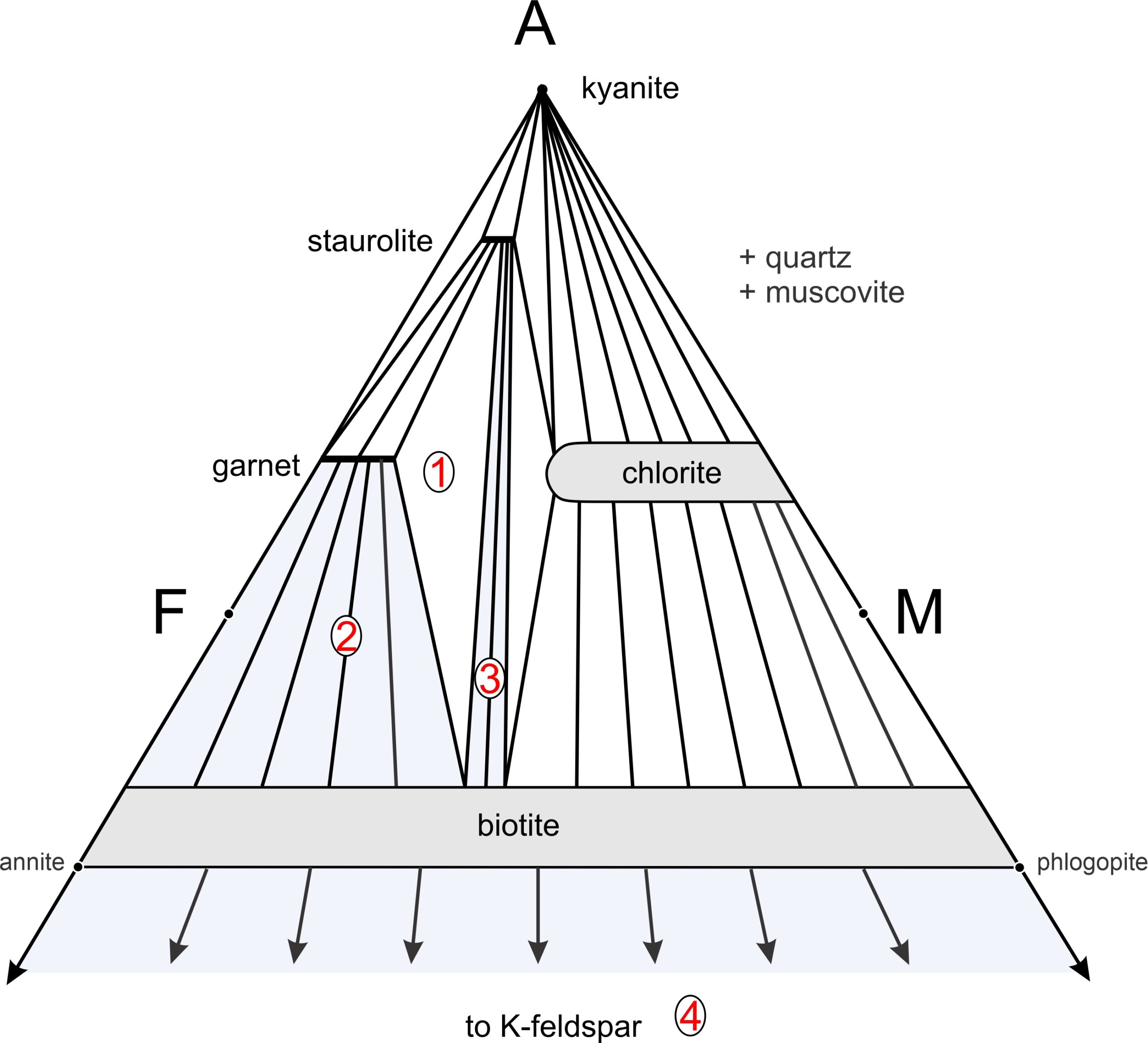
Figure 11.40 is a typical AFM projection for medium-grade metapelites. This diagram depicts stable mineral assemblages at one pressure-temperature condition. We can plot any rock composition on this diagram to learn the stable assemblage. The triangular diagram depicts five possible 1-mineral assemblages, seven possible 2-mineral assemblages (connected by tie lines), and four possible 3-mineral assemblages (shown by white by triangles). Besides the minerals labeled on the diagram, quartz and muscovite (phases projected onto this triangle) will be present. If either P or T change, the diagram may change as new tie lines replace old ones or the size and shape of mineral composition fields vary.
Many medium-grade metapelites contain staurolite, garnet, and biotite (depicted by the white triangle labeled 1 in Figure 11.40) Muscovite and quartz are present with these minerals, too. Plagioclase is also sometimes in metapelites of this grade, but Thompson projections ignore CaO, and thus they ignore plagioclase. Other common assemblages at this metamorphic grade include garnet-biotite-muscovite-quartz without staurolite (the blue field labeled 2), and staurolite-biotite-muscovite-quartz without garnet (the blue field labeled 3). For both compositions 2 and 3, tie lines connect the compositions of minerals that coexist. The arrows from biotite pointing downward to K-feldspar remind us that for some aluminum-poor compositions, biotite-K-feldspar-muscovite-quartz may be the stable assemblage (the blue region labeled 4) without any of the more aluminous minerals.
11.5.5 Suppose Muscovite is Not Present ?
We will discuss one other wrinkle later in Chapter 14. Projection from muscovite works very well for metamorphic rocks that contain muscovite. Muscovite, however, breaks down at high grades of metamorphism, producing K-feldspar and other minerals. Lacking muscovite, however, we can project from K-feldspar. This leads to AFM diagrams very similar to what we have just seen, except that all phases plot within the AFM triangle.
11.6 Petrogenetic Grids and Pseudosections
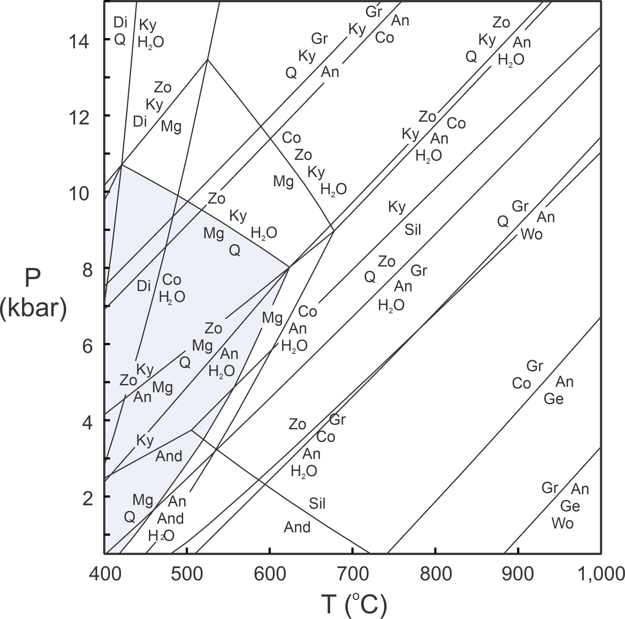
Figure 11.41 depicts the most important reactions that could affect a hypothetical rock containing CaO, Al2O3, SiO2, and H2O components. We call this type of diagram a petrogenetic grid. Grids of this sort apply to a specific chemical system, and to a specific set of phases. If we change the system, or add or subtract minerals, we will get a different grid.
We can use computer programs (discussed in Chapter 12) to calculate diagrams such as the one seen in Figure 11.41. Although different programs yield slightly different diagrams, the results are all quite similar. However, no natural rocks contain only CaO, Al2O3, SiO2, and H2O. FeO and MgO are always present, for example. Adding these additional components will add reactions and complications to the phase diagram. An additional complication arises because, as pointed out earlier in this chapter, individual reactions on phase diagrams only affect rocks of particular compositions. They may not affect some rocks or mineral assemblages at all. Furthermore, if a diagram contains many reactions, it can be difficult to identify those that apply to any particular rock.
Despite some shortcomings, petrogenetic grids like the one in Figure 11.41 can give us valuable information. If a rock contains margarite and quartz (Mg + Q on this diagram), for example, it must have equilibrated in the region highlighted in blue. Other minerals and assemblages are stable only in specific fields on the diagram, too.
If too many reactions, many of which may not apply to a specific rock, are confusing, what about calculating a phase diagram that applies to a rock of one specific composition? We can do this, and the result is a pseudosection, also called an equilibrium phase diagram. Figure 11.42 is an example. We can calculate and plot pseudosections like this one using any of several computer programs discussed in Chapter 12.

Figure 11.42a is the same phase diagram we saw previously (Figure 11.20) for minerals and reactions in the Al2O3-SiO2-H2O system. Figure 11.42b, a pseudosection, appears somewhat like the phase diagram but is different. In the pseudosection, reactions are unlabeled, and field labels show equilibrium mineral assemblages for different conditions. This pseudosection, like all pseudosections, however, is only valid for a single rock composition. In this example, a red asterisk in the triangular inset in Figure 11.42b shows the composition. It is close to the composition of kaolinite and plots within a triangle with diaspore, kaolinite and H2O at the corners.
At low temperature, the hypothetical rock in Figure 11.42b contains diaspore, kaolinite, and H2O. At higher temperature, pyrophyllite forms. With further heating the hydrous minerals (diaspore and kaolinite) disappear, leaving a rock that contains an aluminosilicate (kyanite, andalusite, or sillimanite) with quartz and water.
The lines dividing fields in Figure 11.42b are the same as the reaction lines in the corresponding phase diagram. But some lines in the phase diagram are absent from the pseudosection. This reinforces the notion that not all reactions apply to all composition rocks. If we started with a different composition rock, fields of different shapes containing different assemblages would likely be on the pseudosection.
A key difference between phase diagrams and pseudosections is that we can calculate a phase diagram that describes all possible reactions in a given chemical system. In contrast, if we wish to look at pseudosections, we must calculate a different pseudosection for every composition rock we wish to consider.
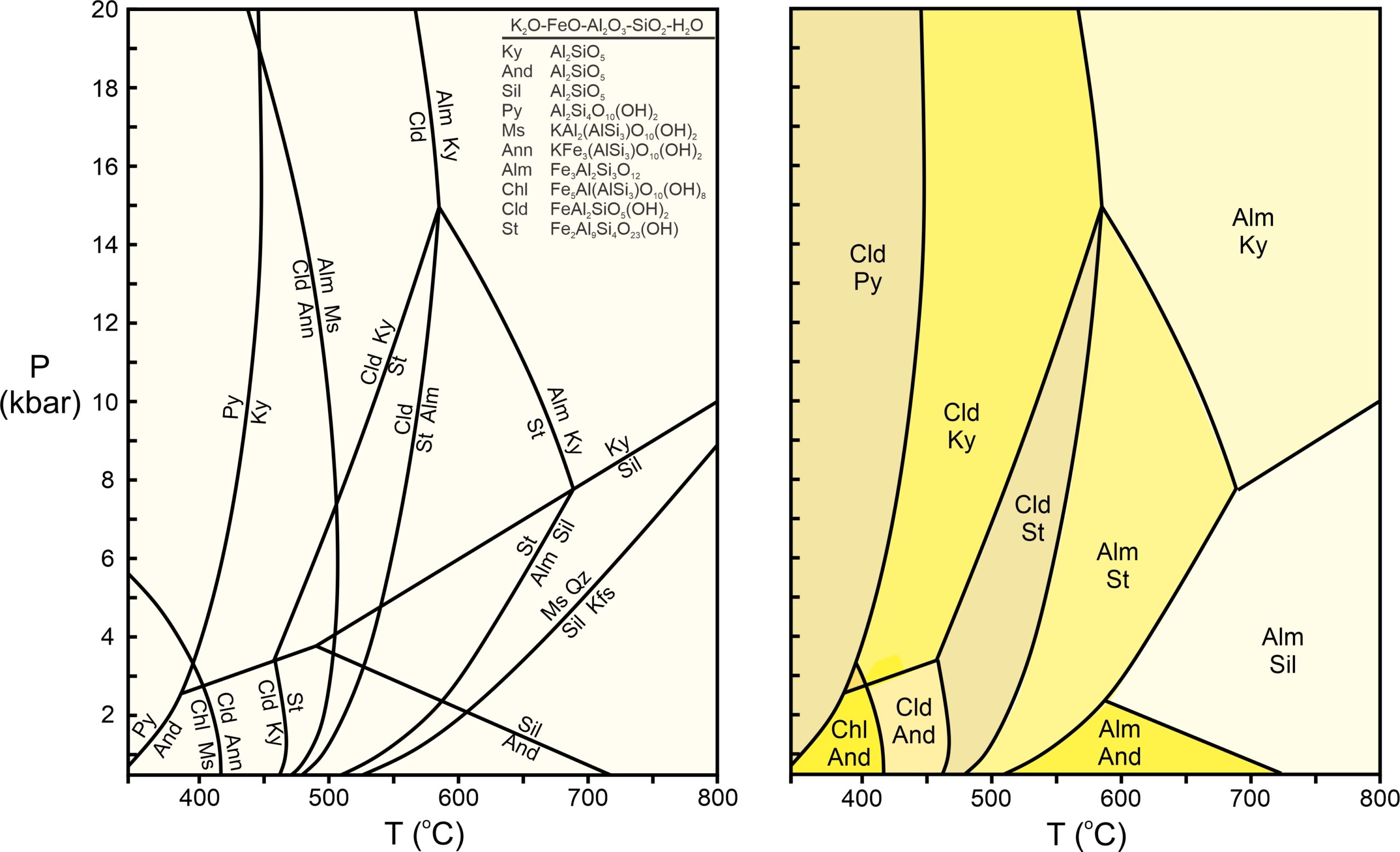
Figure 11.43 is another example of a phase diagram and corresponding pseudosection. The phase diagram displays all reactions in the K2O-FeO-Al2O3-SiO2-H2O system that can occur during metamorphism of a pelitic rock involving the 10 minerals listed. To simplify and avoid clutter, the reaction labels omit any quartz and H2O that are involved (because quartz and H2O are generally present in pelites).
The drawing on the right in Figure 11.43 shows stable assemblages for one composition. This pseudosection shows the same trend we have seen previously in this chapter – the hydrous phases give way to anhydrous phases at elevated temperature.
The diagrams in Figure 11.43, however, do not apply directly to real rocks, because pelites always contain MgO (and often other significant components) not considered in these diagrams. If we added MgO to the system, things would become more complicated because we would gain new minerals and reactions. More significantly, many reactions would become sliding reactions and no longer plot as lines on the phase diagram. We could, however, use computer programs to calculate pseudosections and stable mineral assemblages for any given rock composition. If many components are involved, there will be many more stability fields than the ten seen in Figure 11.43b.
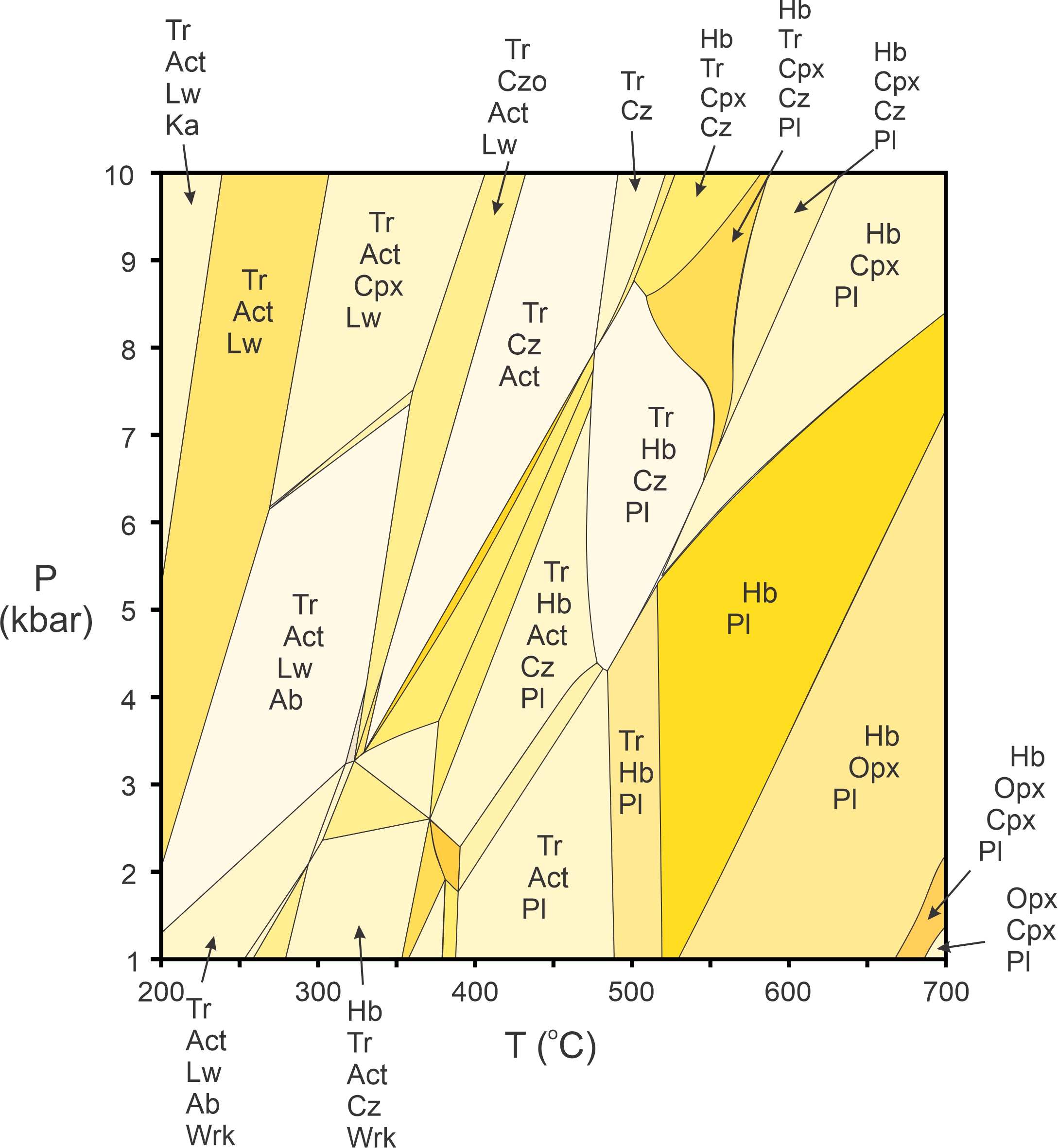
We will not dwell much on complicated pseudosections in this book, but Figure 11.44 is an example. It displays stable mineral assemblages for one composition mafic rock. The section includes all the most common minerals and reactions in the Na2O-CaO-FeO-MgO-Al2O3-SiO2-H2O system. We omitted many field labels to avoid clutter, but the general idea should be clear: in a multicomponent system, the mineral assemblage in a rock constrains the pressure and temperature at which the rock could have formed. Although not shown in Figure 11.44, programs that calculate stable mineral assemblages also calculate the compositions of solid-solution minerals at any pressure and temperature.
So, pseudosections are powerful tools that petrologists can use. A difficulty is, however, that to use the tool requires knowing rock composition and calculating a diagram such as this one for every different composition. While calculating pseudosections is reasonably straightforward with available computer programs, obtaining a rock analysis takes time and sophisticated equipment. Often, petrologists do not have that information.
● Figure CreditsUncredited graphics/photos came from the authors and other primary contributors to this book. 11.2 Weathered granite, lyellcollection.org |